Image Analysis Results
When a run lands, the middle of the workspace switches to what it found. Four tabs at the top of that panel move between the run's views: Viewer, Measurements, Gallery, and Objects.
Viewer
Viewer is the single image you were tuning, full size, with the inspected step's overlay drawn on it and the row underneath to move between images. The tabs appear once a run has covered the set, and until then the Viewer fills the workspace.
Measurements
Measurements is where a finished run opens, and it puts the images side by side. A pipeline that measures several things per image, or every object separately, shows a chart over the table it is drawn from.
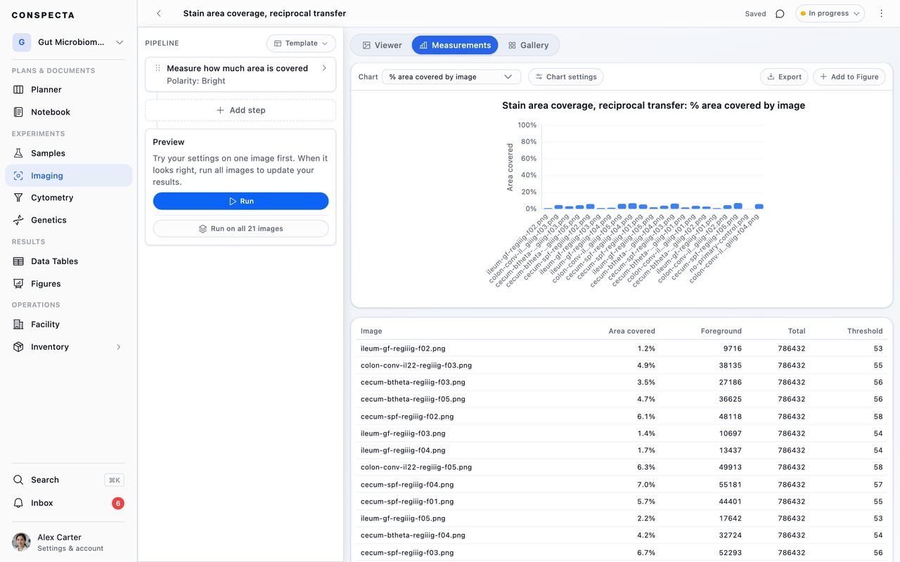
The chart opens on the one that measurement calls for, titled with the analysis and the chart's name:
| A pipeline that | Opens on |
|---|---|
| Measures one number per image, such as a count of objects or the area they cover | One bar per image, with the file name beside it and the value at the end of the bar, so you can read the whole set down the panel |
| Classifies pixels | % positive by image, on a 0 to 100% axis |
| Counts objects inside regions | A dot on every region, with a column per image |
| Measures colocalization | Pearson r by image |
| Measures every object | A box per image over that image's objects, so you read the spread rather than an average of it |
Chart in the bar above the plot lists the charts this run can be drawn as. Other measurements by image at the end of that list plots the numbers the named charts leave out, one at a time. A pipeline whose numbers they all cover doesn't show it, and one nothing recognizes shows Results by image and every number it wrote.
Chart settings beside it opens the chart type and the column picks, so you can take any of these somewhere else. That table draws 50 rows at a time and Show 50 more adds another page.
Column headings read as words, and a fraction like area covered is shown as a percentage. A per-object pipeline writes a row per object, so a dozen images runs to thousands of rows. A z-stack writes a row per focal plane that ran, named for the image and the plane, such as Plate 3 · z4, so a stack trimmed to 13 slices lands as 13 rows rather than one.
Accept run 6 at the foot of the numbers settles them and puts them on a notebook page, as Accepting a Run describes below.
A pipeline that writes one row per image, such as a count of objects, also records what each setting left on Auto came to on each image. Each of those settings gets a column after the measurements, named for the setting, such as Threshold used or Background offset used, and a count shows it beside each image's bar. Read down it to see whether the automatic cutoff moved across the set. The chart, the headline number, and Compare leave these columns out.
Gallery
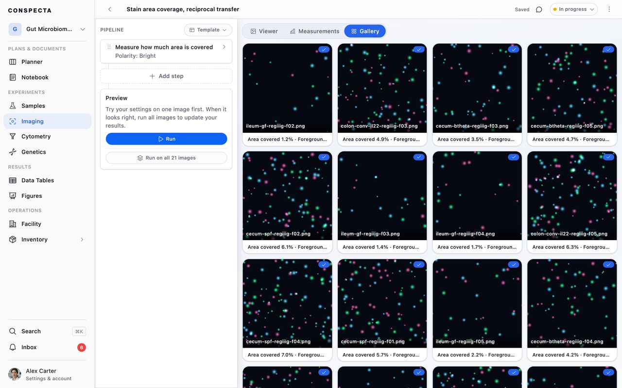
Gallery gives one card per image with its headline number and how many checks fired. Click a card to open that image in the Viewer. An image the pipeline couldn't analyze is named in a band above the cards, with the reason.
Objects
Objects appears when the pipeline detects objects, and shows every one it found as a cut-out across the whole set. With more than one image contributing, Filter by Image narrows the grid to one. After a run on Conspecta's servers, an image's overlay appears when you open it in the Viewer, and its objects join this grid once you have.
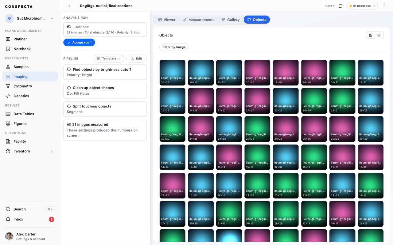
When a filter or the detector threw objects away, the heading counts both, such as 12 kept · 3 rejected, and Show rejected adds them to the grid. A rejected cut-out is grayed, with the reason in place of its size.
Filtered by size, 9 px names the filter that dropped it and the value it was dropped on, so you can see whether your cutoff is landing where you meant. Outside the area counted and Glare are the detector's own, which happen before any filter runs. A run made before Conspecta started keeping rejected objects has no Show rejected, so run the set again to get it.
The Results Table
Every run writes its numbers into a results table automatically. That table belongs to the analysis itself, and the chart, the figure picker and the notebook embed all read from it, so results are one click from a chart and two from a figure.
It takes the analysis's sharing too, so the numbers from an image analysis you keep private stay yours, and sharing the image analysis hands them to the project. To read one run against another, Compare Image Analysis Runs puts several of them into a single table.
Exporting
To take the numbers elsewhere, the ⋮ menu at the end of a run's top bar has Export CSV, which downloads the same rows as a spreadsheet file. It appears once a run has results.
Export in the Analysis tab's header writes the list of every image analysis in the project as CSV or Excel, with each one's name, type, status, how many images went in, how many runs came out, when it last ran, and its headline result. Tick rows first and Download on the bulk bar opens the same dialog box on the rows you ticked, with a ticked folder standing for what is inside it.
Export in the Images tab's header downloads image files. Scope is every collection in the project, or the ones you ticked, which is what Download on the bulk bar opens on, and a ticked collection stands for the images inside it. One image comes down on its own and several as a ZIP, up to 256 MB at a time.
What Produced These Numbers
Once a run has covered the set, the sidebar's steps lock to the ones that run used. Analysis run at the top shows the run whose numbers are on screen, with when it finished and how much it covered.
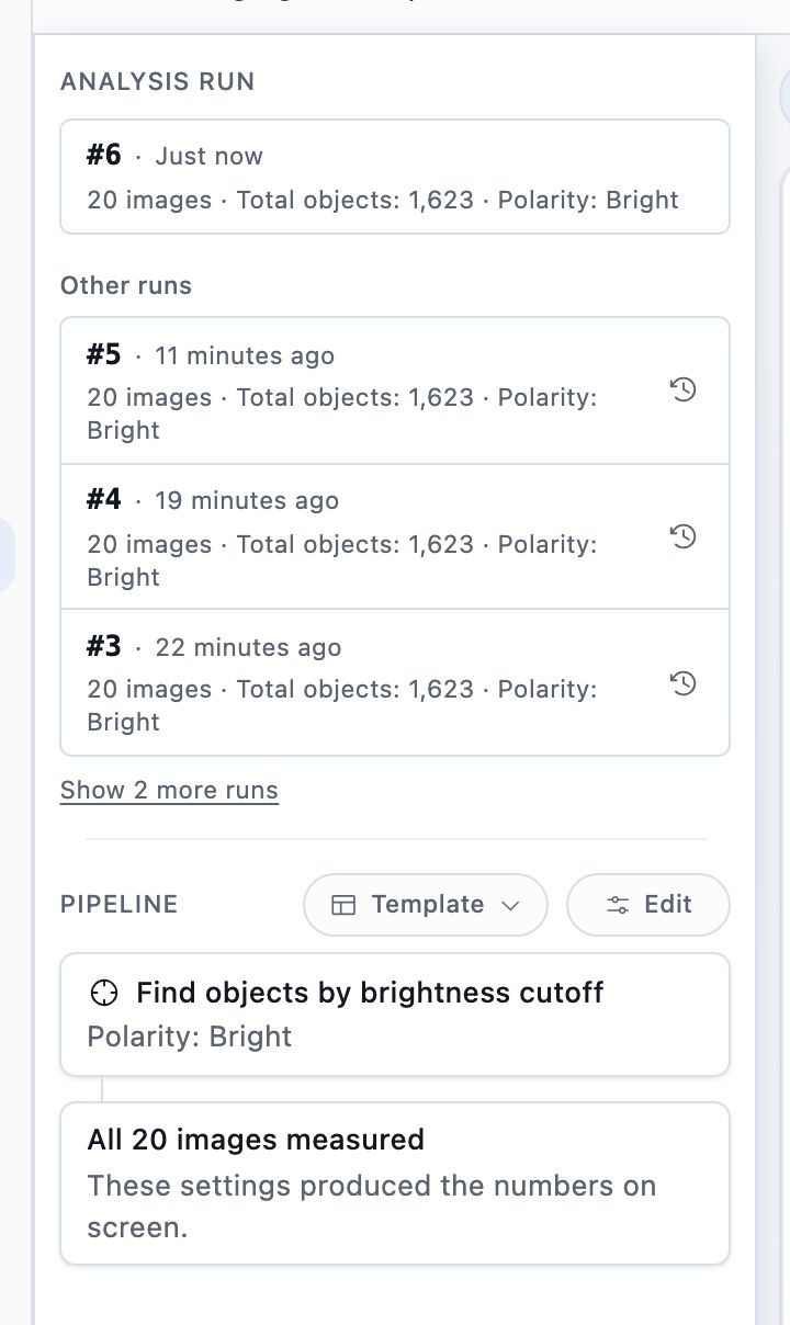
Right after you run the set, Accept run 6 sits under it too, the same button as the one under Measurements. Other runs under it lists this image analysis's remaining runs, newest first and numbered, three at a time, and the link under them, such as Show 2 more runs, opens the rest. Pipeline under it holds the locked steps.
The settings listed there are the ones that produced the numbers beside them. Change a setting without running again and a note appears over the results naming the run that produced them.
Edit, at the end of the Pipeline heading, unlocks the steps where they stand, so nothing in the sidebar moves. The same button then reads Done and locks them again, and running the set locks them too.
Going Back to an Earlier Run
Each run in the list carries its headline number, so you can compare what each one found. Use these settings, the clock button at the end of a run's row, brings that run back: its measurements return to the screen and its steps return to the sidebar.
Nothing runs again, so it takes no compute and adds no run to the list. The run moves to the top of Analysis run, and Accept run 3 at the foot of Measurements now names it, so you can accept the run you came back to.
The buttons show while the steps are locked, so press Done first when you are editing.
Bringing a run back replaces what is in the results table with that run's numbers. A row you typed into the table yourself belongs to no run, so it goes with the rest. To keep one, copy it somewhere else first. To get a later run's numbers back, press Use these settings on that run.
Runs recorded before September 2026 kept no copy of their measurements. On those, Use these settings brings the steps back and says so, and you run the set again to measure it. An image analysis keeps every run it has ever recorded.
Accepting a Run
When the numbers are right, Accept run 6 settles them. It sits at the foot of Measurements and names the run on screen. Right after you run the set it also sits under that run in the sidebar's Analysis run. On an image analysis you open later it waits under Measurements, so you accept a run once you have read its numbers.
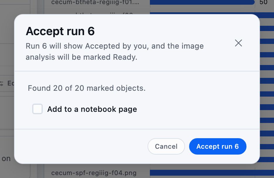
Press Accept run 6 in the dialog box to accept the run on its own. To put it on a notebook page as well, tick Add to a notebook page first, pick a page, and keep Methods ticked for the steps and their settings and Results for the numbers.
The image analysis moves to Ready, the run shows who accepted it and when, and a page you picked gets the steps and a table named after the image analysis and the run, such as Nuclei count (run 6).
The Methods text names the method behind each setting left on Auto and the range it came to across the set, such as "Threshold: Auto (Otsu), resolved to 96 to 131 across 12 images". A set too large to record every image's settings gives the range "on the images recorded" in place of the image count.
That table is a copy, listed in Data Tables with the rest. Later runs rewrite the image analysis's own results table and leave the copy's numbers as they were accepted.
The run whose numbers are on screen is the one that can be accepted, once it has finished, and only once. That is the newest run until you bring an earlier one back with Use these settings, which makes that run the one you can accept. Anyone who can edit the project can accept a run.
The copy is shared with the project when the image analysis is. A private image analysis gets a private copy, so teammates reading a shared page see a placeholder until you share that table from Data Tables. Changing the image analysis's sharing later leaves the copy as it is.
Tip: Reopening a finished image analysis restores its numbers without re-running anything, which uses no compute usage. Measurements and Gallery come back in full. Objects is drawn from the masks a run produces, and those masks are rebuilt by each run and not stored, so Objects fills in for the images you run again.