Manage Genetic Sequences
Genetics is where DNA, RNA, and protein sequences live: imported or fetched, annotated, analyzed, and kept as a library your whole project can reach. This page covers the library itself, getting sequences into it and finding them again.
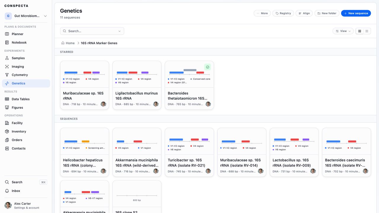
Sequences sit in folders, and every card carries the map of what's in it, so you can find a construct by looking at it. Opening one gives you the map itself, covered in Plasmid Maps and the Sequence Viewer. From there, the tools that read a sequence are in Sequence Analysis and BLAST, the ones that cut and join it are in Restriction Digest and Cloning, and cataloging one as a plasmid or a strain is in The Sequence Registry.
Adding a Sequence
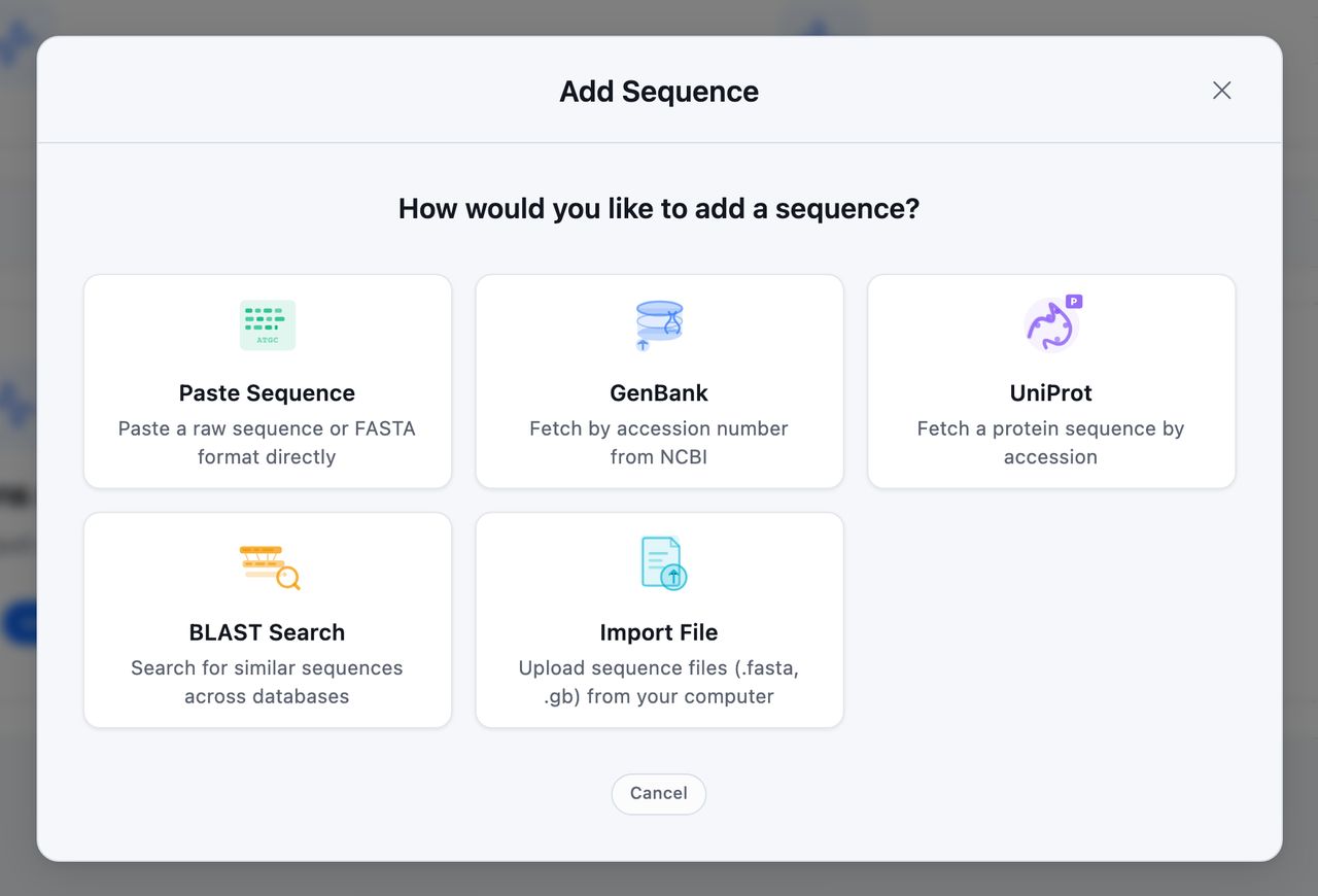
New sequence opens Add Sequence, which offers five ways in:
| Method | What it does |
|---|---|
| Paste Sequence | Paste raw sequence or FASTA text |
| GenBank | Fetch a record by accession number from NCBI |
| UniProt | Fetch a protein by accession |
| BLAST Search | Search for similar sequences and save a hit |
| Import File | Upload FASTA, GenBank, SnapGene, or Sanger trace files from your computer |
Whatever you add lands in the folder you had open when you chose New sequence. Adding a single sequence opens it, and a batch stays in the list so you can see all of it arrive.
Pasting lets you set the Sequence Type, which filters the box to that type's alphabet, so a protein pasted while DNA is chosen loses its residues. Auto-detect keeps any letter a DNA, RNA, or protein sequence can hold and works out the type when you add the sequence. You also choose whether the sequence starts private or shared.
You can paste FASTA text with its header lines. A header names the sequence unless you typed a Name, and a paste holding several records adds one sequence for each.
A GenBank fetch brings the record's annotations and its topology, so a circular plasmid opens on the plasmid map. A UniProt fetch brings the protein sequence, which is everything UniProt returns for it.
Fetching a record sends the accession you typed to NCBI or UniProt, and searching by keyword sends the words you type. Conspecta makes the request for you, so the address those databases see is our server's. Nothing else from your project goes with it, no account, project, or contact details. BLAST is covered in Sequence Analysis and BLAST, which sends more.
Import File takes .fasta, .fa, .fna, .ffn, .faa, .frn, .gb, .gbk, .gbff, .genbank, SnapGene .dna, and Sanger .ab1, several at a time and several records per file, up to 64 MB each. You can also drag files onto the workspace, which imports the batch into the folder you are in with a running count, and those arrive private. A file that brings in one sequence opens it.
Import, under the ⋯ in the header, takes the same FASTA, GenBank, SnapGene, and Sanger trace files as the dialog box's own import step, and a file holding several records becomes several sequences. A SnapGene file keeps its features and its topology, so a plasmid arrives as a plasmid map, and a .ab1 arrives as a read carrying its per-base quality.
Conspecta reads the format from the file's contents, so a .dna that was renamed still imports, and a file that can't be read is named along with the reason. File Formats and Importing lists what each format carries across, and which ones Conspecta turns away.
Organizing Your Library
Sorting and Filtering
View on the toolbar holds sorting and filtering. Each choice shows as a removable label under the toolbar.
| Control | Choices |
|---|---|
| Sort | Date, Name, Sequence Type, or Review |
| Filter | Type, Modified, Owner, and Review |
| The review filter | Review requested, Changes requested, Approved, Rejected, and No review |
The review filter is read from the sign-offs and review requests each sequence carries. An Analysis filter joins them once any sequence in the project is linked to one, so you can pull up everything that fed a particular piece of work.
Folders and Stars
Folders and stars work as they do elsewhere. Starred sequences group above the rest, New folder makes a folder in the one you are in, and dragging a card onto a folder moves it.
Each folder carries its own ⋯ menu, acting on that one folder: Rename, Move to..., Star, Download, Share or Make private, and Delete. A view-only member keeps Star and Download.
Download opens the export dialog box on that folder and everything in it, whichever folder the list is showing.
The visibility entry follows what the folder holds:
- A folder of private sequences is offered Share.
- A folder of shared ones is offered Make private.
- In a large workspace both can show, and whichever you pick covers every sequence in the folder.
Only a sequence's creator can change its visibility, so a colleague's sequence inside the folder keeps its visibility, and a message tells you so.
Bulk and Row Actions
Selecting rows brings up the bulk bar: Rename on a single row, Star, Move, Share or Make private, Download, Align, and Delete. In the list, a sequence's row carries a ⋯ with the same actions for that one sequence, plus Duplicate sequence.
Sequence Details
Inside an open sequence, clicking its name in the header opens Sequence details, which holds the description and tags, the length and topology, where the sequence came from, and when it last changed. A view-only member reads it.
The pencil beside Name renames it, so a name can be corrected while you have the map in front of you. Type the new name and press Save or Enter.
The description and the tags are edited in the same panel. Click either one to open it, press Enter to save and Esc to cancel. A sequence takes up to ten tags.
Duplicating a Sequence
Duplicate sequence in a sequence's ⋯ menu, or in the actions menu at the right of the top bar inside an open sequence, makes a copy in the same folder and opens it. The copy is named <name> (Copy), and a second copy of the same sequence becomes (Copy) (1). It keeps the bases, the annotations, the display settings, the tags, where the sequence came from, and its registry kind and fields, and it takes the original's sharing.
The copy starts its own history. It belongs to you and reads as Draft, with no published versions or sign-offs, and it has no catalog number, since that number names one registered item. Its activity opens with a line naming the sequence it was duplicated from, and the original's activity gains a line naming the copy. Duplicating needs edit access to the project.
Delete sequence, last in the actions menu inside an open sequence, moves it to Trash and returns you to the list. The message that confirms it has Undo, and the sequence can be restored from Trash for 30 days. Deleting needs edit access to the project.
Editing a Sequence Someone Else Has Open
An open sequence saves as you edit it. Two people can work on the same sequence at once, and if you add an annotation while a teammate renames the sequence, both changes stay.
If you both changed the same thing, such as the name or one annotation, a box under the header shows Some fields were updated by another user. with each version under Keep mine and Use theirs. Nothing else you change saves until you choose and click Apply.
When a save doesn't go through, the header reads Not saved with a Retry button. Leaving the page while a change is unsaved asks first.
Signing off, asking for a review, publishing or restoring a version, moving the sequence to another project and duplicating it save your latest change first. If that change can't be saved, while you're offline for example, the action doesn't happen and a message says the sequence couldn't be saved.
Finding a Sequence
The search box above the list matches part of a name, description, registry ID, or tag across the folder you have open and everything inside it, so a sequence filed two folders down still comes back, with its folder trail under its name. The chevron inside it opens Find a sequence, which searches by bases, so you can check whether you already have a sequence.
Paste a sequence, raw or FASTA, and Conspecta finds every sequence containing it across every project you can reach. It matches exactly, as a substring, from four characters up to five thousand. Tick Also search reverse-complement (DNA/RNA only) to search the other strand as well, and a hit found that way is tagged so you know which strand matched. Each result names the sequence, its type, its length, and the project it lives in.
Comparing Two Sequences
Sequence Alignment lines up exactly two sequences and shows you where they differ. Tick two in the list and Align in the bulk bar opens on both of them. Align in the header opens it empty, and you pick both inside.
Either way, choose Global (Needleman-Wunsch) to align them end to end, or Local (Smith-Waterman) to find the best matching stretch.
Two sequences align together when both are protein or both are nucleotide, so ticking a plasmid alongside a protein carries only the plasmid across.
Tick three or more and Align opens Multiple Sequence Alignment instead, with everything you ticked already staged. The same type rule applies, and the first sequence you ticked sets it. Multiple Alignment is also in a sequence's own Analysis menu, covered in Sequence Analysis and BLAST.
Activity and Sign-offs
Every sequence carries an Activity panel with comments and sign-offs, alongside the record of who changed what. @ mentions reach a colleague once the sequence is shared with a project that has other people in it. Select a range of bases before you comment and the comment is anchored to those bases.
A sign-off is against the sequence as it stood when it was given, meaning the bases and their annotations. Editing those flags the sign-off for another look, while a rename or a description edit leaves it standing. When what was signed matches a published version, the sign-off names that version, so "approved at v1.2.0" is part of the record.
The sequence's card shows it as a small colored mark that you can hover to read the status and who approved it, rejected it or asked for changes.
| Mark | Status |
|---|---|
| Green | Approved |
| Amber | A review still owed, changes requested or an edit since |
| Red | Rejected |
The list view and the construct picker spell it out, reading Approved v1.2.0 while the sequence still matches and Approved · edited since once it has been edited.
Publishing Versions
Beside a sequence's name sits the version it reads as:
- It shows Draft until the first publish, then the version number.
- It gains edited once the bases, the annotations, or the name differ from every published version.
- Restore an older version and the badge names that one, even while a newer version stands in the history.
Click it to open version history, which also sits in the actions menu at the right of the top bar.
Version history keeps named copies of the sequence, the way a notebook page keeps published versions. Publish new version takes the name, the bases, the type, and the annotations as they stand and gives them a number, so the construct you cloned from, or the sequence a report cites, stays readable after the live copy changes.
Publishing asks how much changed. Major, Minor, and Patch decide which part of the number moves, the first publish is always v1.0.0, and notes are saved with it so the history says why each version exists, and who published it.
Tip: Publish a version before applying a codon optimization or handing a construct to a colleague. The published copy can't be edited, so that version stays as you published it whatever happens to the working sequence.
Restoring a Version
Opening a version shows the sequence as it was published, bases and annotations included. Restoring one writes that name, those bases, and those annotations back over the live sequence, so you can undo a codon optimization days later, from another computer.
The sequence then reads as the version you restored. It is badged Current in the history and named beside the sequence's name, and the newer versions stay in the list to go back to. Publish the current state first if you want a way back to it. You can publish again from the restored state.
Withdrawing a Version
Withdraw takes a version out of circulation when you published it by mistake or bumped the wrong number. Conspecta asks why, and the answer is required. It sits beside the version from then on, so whoever finds it later knows what was wrong with it.
The version stays in the history marked Withdrawn, its number struck through and your reason beside it, and you can still open it and read the bases it froze. The sequence falls back to the newest version that still stands, and the withdrawn one can no longer be restored.
Withdrawing is permanent and uses up the number, so after withdrawing v1.1.0 your next minor version is v1.2.0. To bring those bases back, publish them again as a new version.
Downloading
Export, under the ⋯ in the workspace header, and Download in the bulk bar open the same dialog box, and Download opens it on the sequences you ticked. Anyone who can open the workspace can run it.
What comes first, and it decides the rest of the dialog box:
- The sequences themselves writes the bases. FASTA carries the sequence alone, which is what an aligner, a primer tool, or a sequencing vendor expects. GenBank carries the annotations and the topology with it, so a plasmid opens as a map in SnapGene, Benchling, or ApE. One sequence comes down as a single file, and two or more as a zip.
- A list of them writes one row per sequence, carrying what the workspace's list shows about it. This adds Columns, a grouped checklist covering the name, folder, molecule type, length, GC, annotation count, where it came from, and the record, with All and None, and a Format of CSV or Excel with an Export Info sheet naming the project, scope, and filters.
Scope applies to both: this folder only, this folder and everything inside it, the whole workspace, or the sequences you ticked, each with a live count. A ticked folder stands for the sequences inside it.
For a picture of a sequence, use Export Figure inside it, covered in Plasmid Maps and the Sequence Viewer.