Flow Visualization and Compensation
Plots are how you read a Cytometry analysis. This page covers adding plots, setting their type and axis scales, coloring and overlaying populations, and applying compensation to remove spillover from your data.
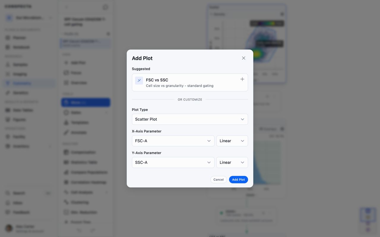
Adding a Plot
When you first open a file, Conspecta adds a starting plot, a density plot of FSC against SSC when the file has those channels.
To add another plot:
- Click Add Plot at the top of the Tools section in the sidebar, or press
A. - Click one of the suggested plots, or set up your own under or customize.
The suggestions come from your panel, such as FSC against SSC for size and granularity, FSC-A against FSC-H for doublet discrimination, and a histogram. Under or customize you choose the plot type, both axes, and the scale of each axis.
Once you have drawn a gate, Population appears at the top of the dialog box. It sets which population the new plot shows, and everything below it applies to that population. This lets you open a plot inside a gate here, as well as with New Plot on the gate itself.
When the Plot Is Already Open
A plot is defined by its population and its pair of channels. Plot type doesn't count, so a density plot and a scatter plot of the same population on the same channels are the same plot.
- Suggestions for plots that are already open are left off the list.
- If the plot you set up by hand is already open, the dialog box says so and its button reads Go to plot, which takes you there. Duplicate beside it adds a copy you can gate separately.
Plot Types
Choose the type from the menu at the top left of any plot.
| Type | Use it for |
|---|---|
| Scatter | Individual events, best when you have few of them |
| Density | Event density as color, the usual choice for gating |
| Contour | Density as lines, which reads well in print |
| Histogram | One parameter's distribution |
Histograms plot % of Max, so you can compare distributions with very different event counts.
A histogram of the Time channel plots the event rate across the run instead, so a clog or a pressure drop shows as a dip. Where other histograms show CV, it shows the run's length and mean rate, such as 12.4 s · 810 events/s.
On a Lin axis the Time histogram reads Events per second against Time (s), or minutes for a long run, when the file records how long each tick of its clock lasts and every file on the plot shares that clock. Otherwise it reads Events per bin against the clock's raw ticks.
Axis Scaling
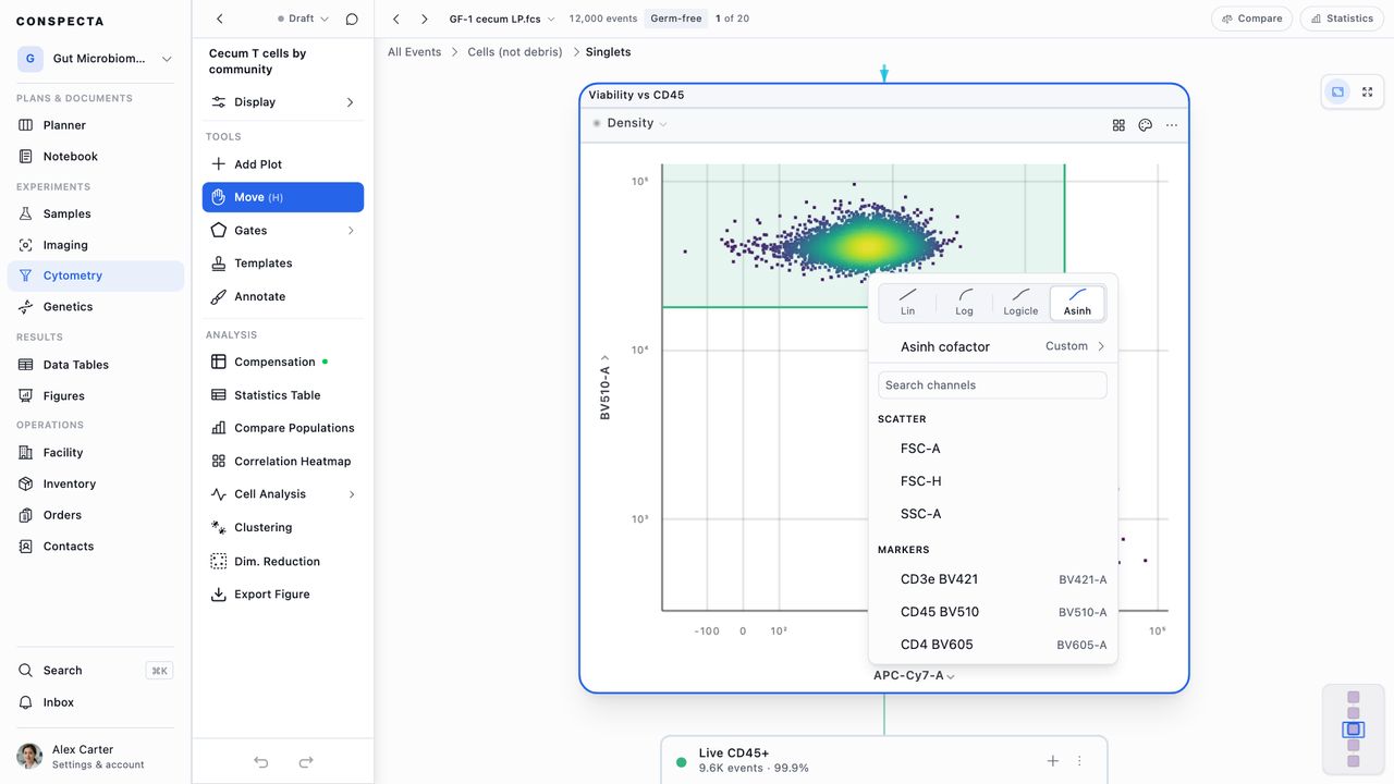
Click an axis label to change its channel or its scale. The menu has two parts:
- The four scales, Lin, Log, Logicle, and Asinh, sit across the top.
- Below them are the file's channels, grouped under Scatter, Markers, Computed, and Other. Each channel is named by the marker it measures, with its detector beside it (CD4 next to FITC-A).
When the file has more than a handful of channels, type in Search channels to narrow the list, and press Enter to pick the first match.
Use Logicle for compensated fluorescence. It is linear near zero and logarithmic above it, so events at or below zero after compensation stay spread out where you can see them. FlowJo draws the same scale, so a gate you draw here sits where you'd expect, and a gating strategy imported from a .wsp keeps the axis it was drawn on.
Adjust the Logicle or Asinh Curve
Pick Logicle or Asinh and a Logicle curve or Asinh cofactor row appears under the scales. It reads Default or Custom. Click it to open the numbers that shape the curve:
- For logicle, Top of scale (T), Linear width (W), Decades (M), and Extra negative decades (A)
- For asinh, Cofactor
A plot imported from a .wsp shows the values it came with, ready to check against the FlowJo file or correct.
Above the fields, the plot's events are drawn on the curve, with the axis's tick labels and a dashed line at zero. The picture redraws as you type, so you can watch a population squashed against zero spread out before you apply the change.
Edit the values and click Apply, or press Enter in any field. The axis reshapes, and every gate evaluated on it moves with it. If you close the menu without applying, your edit is discarded. Reset to defaults puts the standard curve back. The back arrow, or Escape, returns to the scales and channels.
Scale is set on each plot separately. Changing it on a parent plot leaves its child plots as they are.
Reading and Coloring a Plot
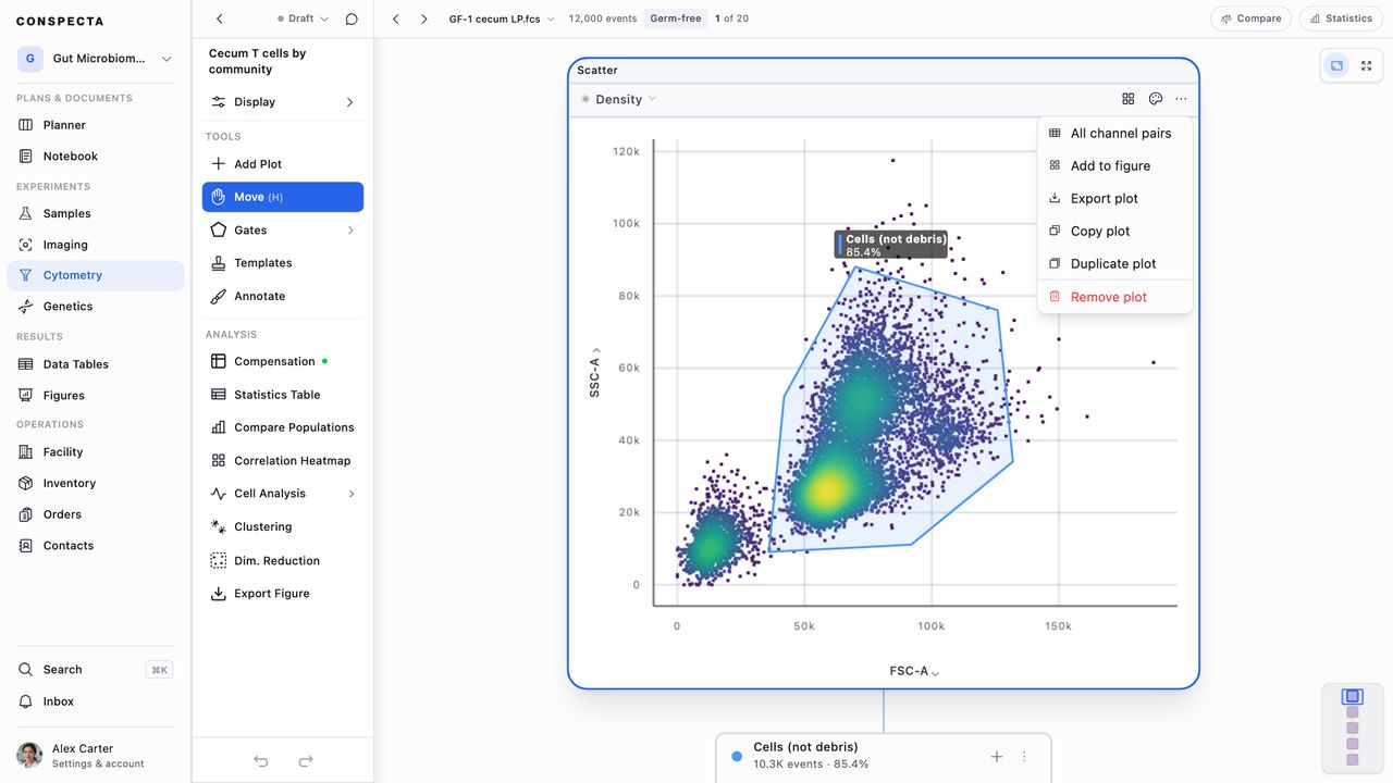
Each plot's header has two buttons on the right. The palette icon, Plot style, sets how the plot is drawn. The ⋯ button, Plot actions, holds what you can do with it.
Plot actions lists All channel pairs, Add to figure, Export plot, Copy plot, Duplicate plot, Paste plot here once you have copied a plot, and Remove plot.
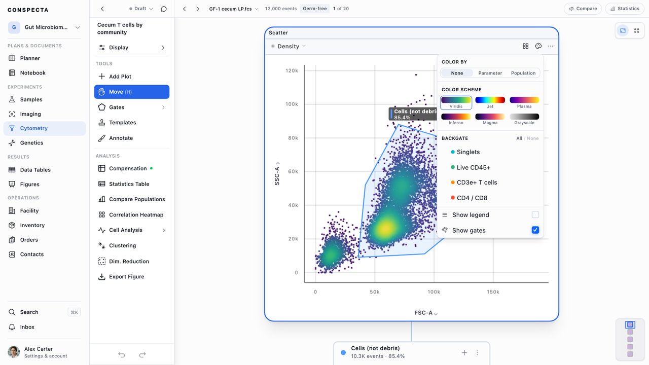
Change How One Plot Looks
Everything in Plot style applies to that plot alone.
- Color By colors events by None, Parameter (a parameter's value), or Population (the population each event falls into). Population appears once the analysis has gates.
- Color Scheme appears on density and contour plots, and whenever you color by parameter.
- Backgate lists the populations gated beneath this plot. Click one to overlay it on the plot, or click All or None beside the heading to add or clear them all. Once a population is on, the arrow at the end of its row lets you change its color.
- Show legend turns the key on or off. On a density or contour plot, turning it on here also shows the Low to High color ramp on that plot.
- Show gates turns the gate outlines on or off. Turn it off to keep a clean copy of a population with no outlines over it. Drawing a gate on a plot with Show gates off turns it back on.
Change Every Plot at Once
Display in the sidebar holds the settings every plot shares.
- Events drawn per plot caps how many events each plot draws, at 10k, 50k, 100k, or All. The default is 50k. Raise it before you draw a gate around a rare population in a tail.
- Color scheme shows six color ramps. Viridis is the default and the one to use in a paper. The others are Jet, Plasma, Inferno, Magma, and Grayscale.
- Show legend turns the key on or off.
- Show density scale adds the Low to High color ramp to density and contour plots. It starts off, and is unavailable while Show legend is off.
A change here updates every plot except the ones you styled by hand in Plot style. Display says how many plots have their own styling, and Match them to these settings brings them back in line.
Scatter, density, and contour plots draw a sample of events up to the cap. Counts, percentages, and every statistic always use every event. The cap changes only what you see.
When the cap leaves events out, the plot's header shows the count beside the plot type, such as 50k of 2.4M. Check it before a plot goes into a figure, because a capped plot looks the same as a full one. Plots too small to fit the count leave it out, which is most of them when you fit the whole tree in the window.
Overlay Populations or Files on a Histogram
A histogram's header has two more buttons:
- Overlays stacks other populations on the same axes, to show a shift between gates.
- Files overlays the same plot from other files, to show a shift between samples. Every file is drawn on one axis wide enough for all of them, and shows the same population the plot does. On a gated plot, a file appears once that gate has been counted in it.
Tip: To overlay populations on a scatter, density, or contour plot, open Plot style and set Color By to Population, or turn them on under Backgate.
Duplicating a Plot
Duplicate a plot when you want the same population twice, such as once on a linear axis and once on log, a density beside a contour, or two gating attempts side by side. Click Duplicate plot in the plot's Plot actions menu, or Duplicate in the Add Plot dialog box when the plot you asked for is already open.
The copy starts with the original's gates, plot type, axis scales, and coloring. From then on the two are separate. Move, rename, or delete a gate on one and the other stays as it was, so a tighter gate and a looser one can sit side by side with their own numbers.
- The gates on the copy are new populations, counted separately. A child plot you open under one of them belongs to that copy alone.
- Only the gates drawn on the plot itself are copied. Populations gated further down stay with the original.
Without duplicating, a gate belongs to its population. Two plots of the same population on the same channels show the same gates, and editing a gate on one changes it on both. Duplicate a plot to get a separate set.
Copying a Plot
Copy a plot to reuse its setup (plot type, channels, scales, and colors) on another population. Click Copy plot in Plot actions, or press Cmd/Ctrl + C with the plot focused.
Copying also puts a picture of the plot on your system clipboard, ready to paste into a slide, a message, or a notebook page. The picture is drawn light on white in either theme.
To paste the setup, click Paste plot here in the Plot actions menu of the plot whose population you want, or press Cmd/Ctrl + V. The keyboard pastes onto whatever you have selected:
| What you have selected | Where the plot lands |
|---|---|
| A plot | On that plot's population, beside it |
| A gate on a plot | On that gate's population, one tier down |
Select a gate and paste to get the same view of the population inside it, without picking channels and scales again on the way down a branch.
- A pasted plot has no gates, ready for you to gate. Duplicate plot copies the population and its gates as well as the view, so use it for two gating attempts on the same cells.
- The copy stays available until you copy another plot, so you can paste the same view onto several populations in a row. You can also paste it into another analysis in the same browser tab.
- Channels are matched by name. Pasting a CD3 against CD4 plot into a sample whose panel is in a different order still gives you CD3 against CD4. If the new sample has no channel by that name, the plot still lands and a message names the channel to check.
Scanning Every Channel Pair
With a many-color panel, hunting for the next gate one plot at a time is slow. All channel pairs in a plot's Plot actions menu opens a dialog box that draws every pair of the selected channels against each other, for the population that plot shows. Each cell is one pair, and the diagonal shows each channel's histogram. A cell where the cloud tilts or splits is a pair worth adding as its own plot.
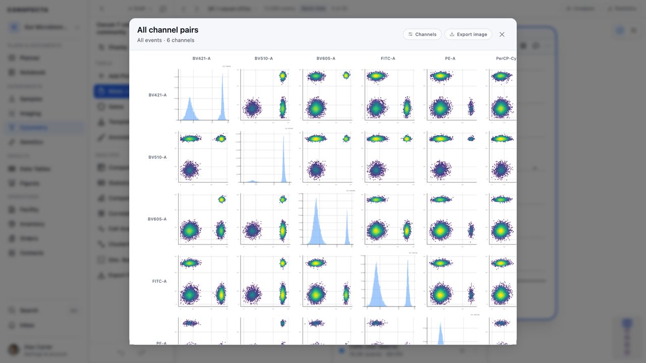
Channels picks what the grid draws. It starts with your first six fluorescence channels and takes up to ten, which makes a grid of 100 plots. Export image opens the grid with two tabs: Export sets the format, size, and file name and downloads or copies it, and Annotate marks it up first.
Navigating a Large Tree
The plots on the canvas are your gating tree. Analyze Flow Cytometry Data covers building one.
- Two buttons in the top right corner of the canvas move the view. One zooms in on the selected plot (
F), and the other fits every plot back in the window (O). They appear once you have more than one plot. - On a zoomed-out tree, click or tap a plot, or the box on an arrow between plots, to zoom in on it. Its buttons work once you're zoomed in.
- The arrow keys move from plot to plot along the gating tree, following the hierarchy instead of their position on screen. Hold
Shiftto stop at the arrows between plots, where each gate's name and count sit.Shift + ↓zooms in on the next arrow down andShift + ↑on the next one up. - On a large tree, a small map of it appears in the bottom right corner. Click a plot's box on the map to focus that plot, or click the space between boxes to move the view there.
- The path above the plots shows the gating route to the selected plot.
Compensation
Click Compensation in the Analysis section of the sidebar. The dialog box has two tabs:
- Matrix holds the numbers.
- Controls holds the tubes they came from, and the check that the matrix corrects them.
A view-only member sees the Matrix tab only.
Read, Edit, or Import the Matrix
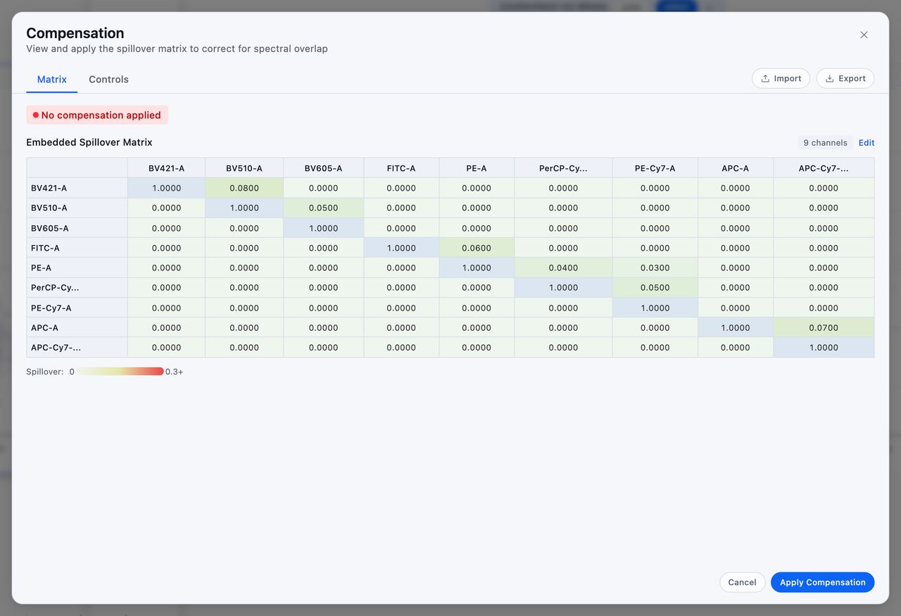
If the file carries a spillover matrix from the cytometer, it is already on the Matrix tab as a heatmap. Click Edit to change the values in a table. Any value above 10% is shaded amber, so an obviously wrong number stands out before you apply it.
The matrix corrects each file's channels by name. If a channel in the matrix matches no channel in some of the analysis's files, a notice above the matrix names that channel and those files, so you can check the matrix before you apply it.
| Button | What it does |
|---|---|
| Apply Compensation | Applies the matrix to the data. It reads Apply Edited Matrix while you're editing, and Re-apply once compensation is on |
| Remove Compensation | Puts the raw data back |
| Import / Export | Reads a matrix from a CSV file, or saves the one you're using |
Tag Your Controls
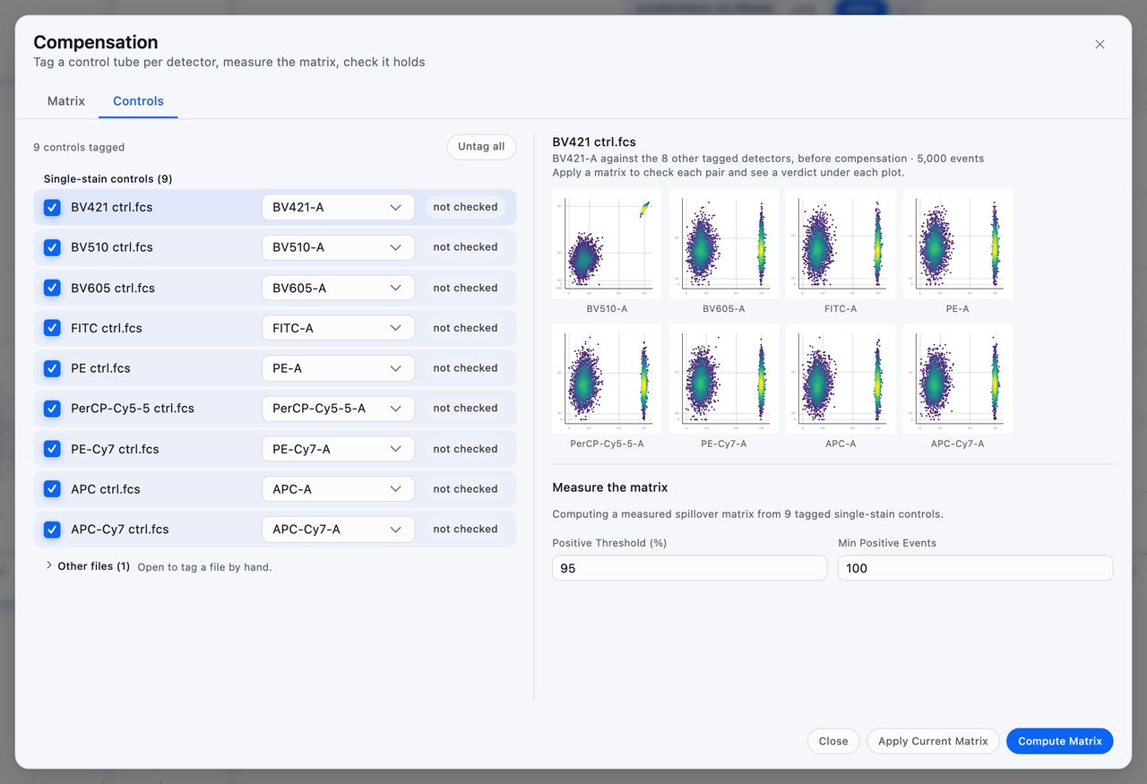
The Controls tab has two sides. The list of files is on the left, and the pane on the right holds the selected control's plots and the matrix you measure. Before a matrix is applied, the plots show the control's events uncompensated, so you can see the spillover the matrix has to remove. Once it is applied, they become the check. Click a tagged file's name or its not checked label to show it in the pane.
Files whose name points at a detector, such as "FITC ctrl.fcs", lead the list under Single-stain controls, with that detector in gray beside each one. The line above the list counts them, such as "9 files name a detector." Click Tag 9 matched controls to tag every one of them at once (the number is how many files it will tag). The line then reads "9 controls tagged", and Untag all takes every tag off again.
Everything else, such as study tubes and an Unstained tube, is folded into Other files. When no file names a detector, every file is listed together instead. To tag a file by hand:
- Tick the file.
- Pick the detector its tube was stained for.
Files that aren't loaded are listed too, with a Load button. A tag only names a detector, so you can tag them now and they are measured and checked once loaded. Tags save with the analysis, so you set them once per experiment.
Each detector can be tagged on one tube only:
- A detector another tube already has reads (taken) and can't be picked.
- A second file whose name points at the same dye, such as "FITC ctrl rerun.fcs", is left untagged for you to place, by a tick and by the tag-all button alike. The detector beside it reads (taken).
- If two saved tags claim the same detector, the row that lost it names the tube that has it, and that tube is the one measured.
Compute the Matrix
The pane beside the list says which data the matrix will come from:
- With at least two tagged controls loaded, Conspecta measures spillover from them. This gives the more accurate matrix.
- With fewer, it approximates the matrix from the open file, and the line names any tagged file it can't use yet.
Two values under that line shape the measuring. Positive Threshold (%) is how bright an event must be to count as positive, and Min Positive Events is how many positive events each channel needs.
Click Compute Matrix and the result appears in the pane. Channel Quality lists each channel's positive-event count and its maximum spillover, and colors any channel whose control is weak or unusable. Below it, a preview of the matrix shows values above 10% in red. Measuring needs at least two fluorescence channels. With fewer, you see a message in place of a matrix.
The button you get to apply the matrix depends on the controls:
| What the controls look like | The button |
|---|---|
| Every control usable | Apply Matrix |
| A control that isn't a measurement (almost no positive events, no signal in its own detector, or more spillover into another detector than into its own) | Apply is turned off, with the reason and the control's name beside it. Re-tag or replace that tube and click Compute Again |
| A control under the minimum you set | Apply Anyway, shown as a secondary button. The matrix is usable but noisier, and applying it is your call |
Check It Worked
Applying from the Controls tab leaves the dialog box open, so you can check the result. The button changes to Applied, and the line beside it reads Compensation applied. It turns back into Apply Matrix when you compute again or change a tag.
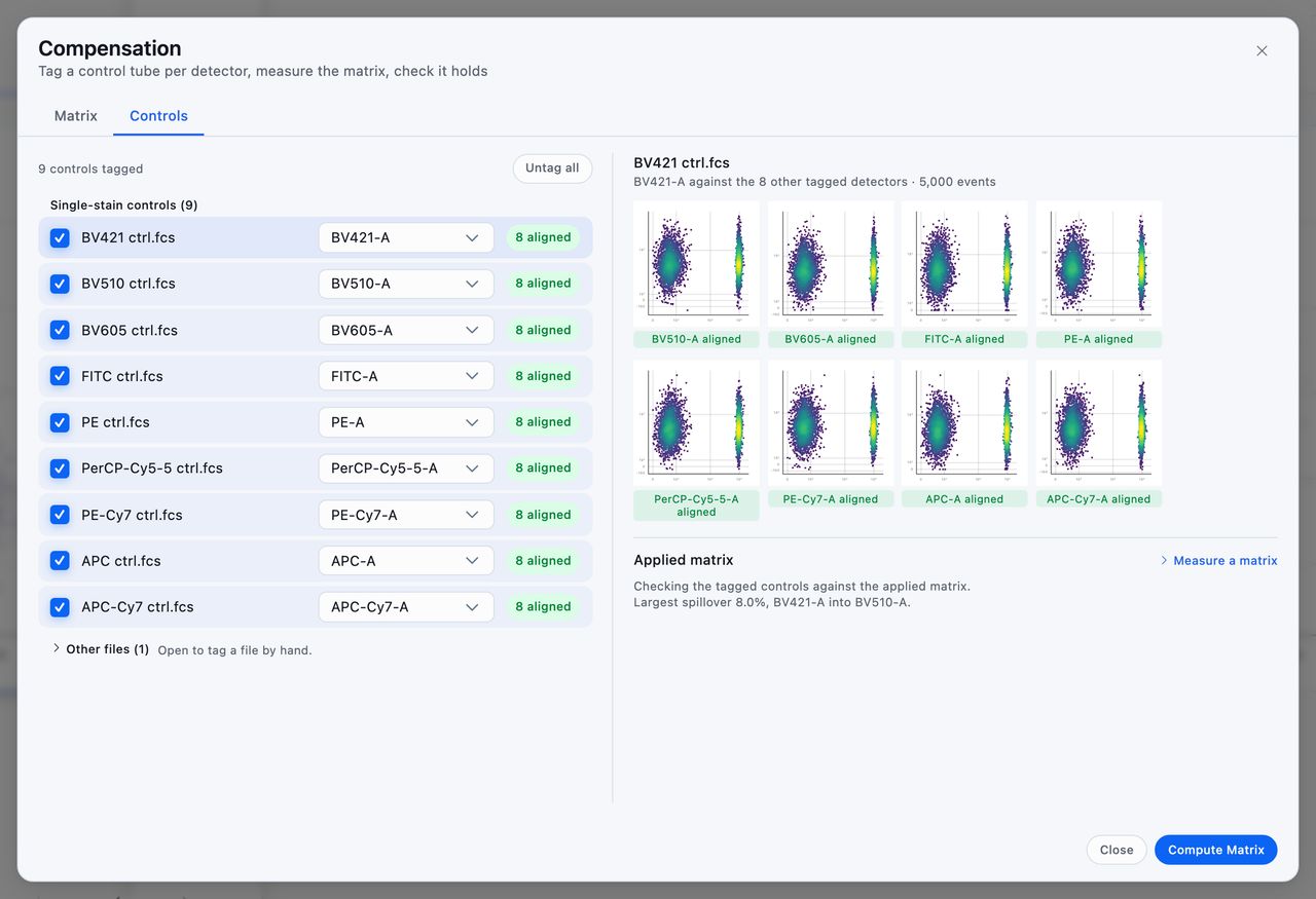
Once a matrix is applied, each tagged control carries a verdict beside its detector:
| Verdict | What it means |
|---|---|
| 8 aligned, in green | Every pair is level, and the number counts them |
| 1 to fix, in red | That many pairs still leak |
| not enough events | The control has too few events to judge |
| tag another | It is the only tagged control, so there is no other detector to read it against |
| not checked | No matrix is applied yet |
| load to check | The file is tagged but not loaded |
Click a file's name or its verdict to show its plots in the pane. Each plot is the control's stained channel against another tagged detector, compensated, with a verdict under it:
- aligned, in green, means the cloud is level.
- under-compensated or over-compensated, in red, names the pair that still leaks, and whether the matrix corrects too little or too much.
- not enough events, in gray, means the control has too few events on that pair to judge.
On a phone, tap a verdict and the plots open over the list.
Under the plots, two lines say where the matrix came from and name its largest spillover. Click Channel quality and matrix to see the measured matrix again. Until you compute a matrix in the dialog box, the same button reads Measure a matrix. Fix a red pair's value on the Matrix tab, apply again, and the plot's verdict turns green.
If you already have a matrix that isn't applied, Apply Current Matrix applies it without computing a new one.
What Applying Changes
Compensation is one setting for the whole analysis, so the axis menu lists the same channels whether it is on or off. Your gates keep the bounds you drew, but the events inside them are recounted on the corrected values. Population counts and percentages change when you apply or remove a matrix.
When a file carries a spillover matrix that hasn't been applied, a banner above the plots reads Compensation not applied, with View and Apply buttons. Dismiss it if you're leaving that matrix off on purpose.
After you click Apply, the banner reads Compensation applied for a few seconds, with an Undo button that takes the matrix back off. Once compensation is on, a green dot appears beside Compensation in the sidebar.
Changing compensation clears saved cell-cycle, proliferation, kinetics, quality-control, and clustering results. Those results were computed on the old values and no longer match the data. Compensate first, then run them.
Annotating and Exporting the Tree
Annotate in the sidebar's Tools section draws text, arrows, and shapes on the canvas, over your plot tree. Use it to turn a gating strategy into a slide. The marks save with the analysis and come back the next time you open it.
To move a mark, choose Move in the Tools section and click the mark to pick it up. Drag its handles to resize or rotate it.
Export Figure in the Analysis section opens the figure with the export options beside it. Choose what to capture (Whole layout, Selected plot, Contact sheet, or Every plot), then set the size and format. Its Annotate tab draws on the figure you're about to export, for that one file only.
To export one plot, click Export plot in its Plot actions menu. Flow Reporting and Export covers every export option.