Analyze Flow Cytometry Data
In Cytometry you upload FCS files, draw gates, compensate, cluster, and pull statistics out, all in the browser.
The Flow Cytometry page has two tabs. FCS Datasets holds your files. Analysis holds the gating you build from them. Accounts in the panel design beta also get a Panels tab, covered in Design a Flow Cytometry Panel.
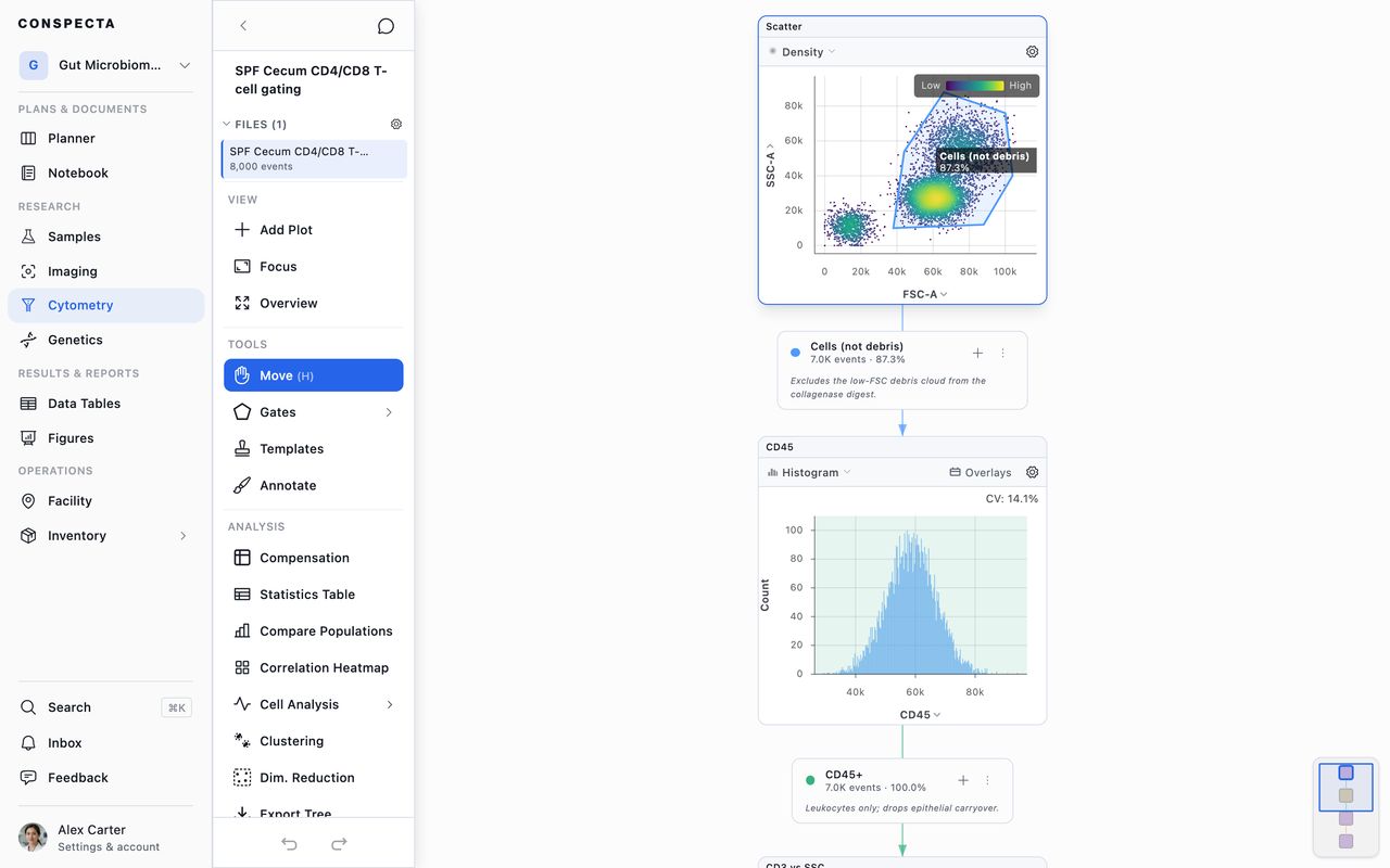
This page covers building an analysis from your files and gating it. To get your files in, attach them to samples, or bring in gating from FlowJo, see Upload FCS Files and Import Gating.
Creating an Analysis
An analysis is where you gate your files. The same FCS files can be in more than one analysis, and one analysis can use files from more than one dataset.
- Click New analysis.
- Enter a name, choose private or shared, and pick the datasets to include.
- Click the create button. It shows the number of files, such as Create analysis with 12 files.
If a dataset you picked is still uploading, the create button stays unavailable and a line under it shows the upload's progress, such as Uploading 8 of 12. The analysis then starts with every file in the dataset.
To sort the list on the Analysis tab, or filter it by review state, click View. The Review filter offers Review requested, Changes requested, Approved, Rejected, and No review, based on the sign-offs and review requests on each analysis.
Large projects show a Load more at the bottom of the Analysis and FCS Datasets tabs. Searching, filtering, opening a folder or dataset, and Export always cover the whole project. Until everything has loaded, a folder's count shows how many have loaded so far, such as 12+ items.
Duplicating a Flow Analysis
Duplicate flow analysis in an analysis's ⋯ menu on the Analysis tab makes a copy in the same folder and opens it. The copy is named <name> (Copy), and a second copy of the same analysis becomes (Copy) (1).
It keeps the files, the gates, the plots, the compensation, the per-file gate changes, the parameter names, the notes, and the template it was built from, and it takes the original's sharing. It reads the same files, so it stays under the same panel version as the original.
The copy starts its own history. It belongs to you and reads as Draft, with no sign-offs, no clustering runs, and no statistics, so run those again on the copy when you need them. A plot the original colored by clusters stays in the layout and takes its colors from the next clustering run.
The copy's activity opens with a line naming the analysis it was duplicated from, and the original's activity gains a line naming the copy.
A dataset on the FCS Datasets tab has no Duplicate flow analysis. Duplicating needs edit access to the project.
The Workspace
Move Around the Canvas
Your plots sit on one canvas in the middle of the screen, arranged as a tree and joined by the gates between them.
- Drag to pan, and scroll to zoom. On a touch screen, drag with one finger and pinch to zoom.
- On a large tree, use the minimap in the corner.
- With more than one plot, two buttons in the opposite corner, above the tree, focus the selected plot (
F) or fit every plot in view (O). They're hidden on a phone. - When the tree is zoomed out too far to use a plot's buttons, click or tap the plot to zoom in on it. Its buttons and gates work once it's large enough, which on a touch screen means close to full size.
- Add Plot is the first item in the Tools section of the sidebar.
Switch Between Samples
A bar across the top of the canvas shows which sample the plots are drawing. It has:
- arrows to the previous and next sample
- the sample's condition and event count
- its position, such as 3 of 12, and how many files aren't loaded
- Compare and Statistics, once more than one sample is loaded
Click the sample's name to open the full list, with Load all and Manage files under it. An analysis with only one sample has a shorter bar, with the sample's name and the same list.
On a phone the bar takes two lines. The first has the back button, the tools, and a menu with Compare, Statistics, and Activity. The second has the sample's name and the arrows, with the sample's position between them. The condition and the files that aren't loaded are in the list. Turn the phone sideways to fit everything on one line.
Rename a File
- In the sample list, open a file's menu and choose File Info.
- In File Information, click the pencil beside Name.
- Type the new name and click Save, or press
Enter.
The new name follows the file into your datasets and every other analysis that uses it. The name the cytometer wrote stays with the file as its original name.
A FlowJo workspace import pairs its samples with your files by name, and compensation uses file names to match each single-stain control to its channel. After a rename, either one may ask you to pick the file yourself.
Find Your Tools in the Sidebar
Once the analysis has a plot, Display in the sidebar opens settings that apply to every plot at once: Events drawn per plot, Color scheme, Show legend, and Show density scale. The rest of the tools are in two sections:
| Section | What's in it |
|---|---|
| Tools | Add Plot, Move, the Gates menu, Templates, and Annotate |
| Analysis | Compensation, Statistics Table, Compare Populations, Correlation Heatmap, Cell Analysis, Clustering, Dim. Reduction, and Export Figure |
Flow Reporting and Export covers the statistics and export tools in the Analysis section.
Set the Analysis Status
The status is in the sidebar's header, beside the Activity button. Click it to change it:
- Draft for an analysis still taking shape. Every new analysis starts as Draft.
- In progress for one you're working through.
- Ready for one you've finished and the rest of the project can use.
The status also shows on the analysis's card and row on the Flow Cytometry page. Each change is recorded in Activity under your name. A member with view-only access sees the status but can't change it.
Once someone has asked for a review or signed off the analysis, a small mark appears beside the status:
- green when it's signed off
- amber when a review is still owed, changes were requested, or the gating was edited after it was signed
- red when it was rejected
Hover the mark to read it in words, or click it to open Activity.
A sign-off covers the gating: the gates and plots, the compensation and its control files, the files in the analysis and their conditions, a gate customized for a single file, renamed parameters, and the shapes and text added with Annotate. Changing any of those marks it edited since. Renaming the analysis, editing its notes, dragging a gate's label or switching the file on screen leaves it approved. The mark on the analysis's card and the one in its Activity panel read the same way.
Undo and Saving
Undo and redo are at the bottom of the sidebar. Cmd/Ctrl + Z undoes and Cmd/Ctrl + Shift + Z redoes. Undo covers every change to the analysis, including gates, plots, axes, channel names, compensation, templates, and a gate customized for a single file. Loading and removing files can't be undone. Undo takes back your own changes and leaves a teammate's gates and plots in place.
Everything saves automatically. The bar above the plots reads Saving… and then Saved.
A large file shows a preview first, so you can start drawing while the rest loads. Statistics always count every event in the file.
Gating an Analysis Someone Else Has Open
Two people can gate the same analysis at once. If you each add a gate, both stay. A teammate's saved changes appear in the analysis you have open without a reload, and on the Analysis tab. Shapes and text a teammate adds with Annotate show the next time you open the analysis.
If you both changed the same gate or plot, a box above the plots shows Some fields were updated by another user. with each version under Keep mine and Use theirs, named by the gate, such as Gate "CD4". Nothing else you change saves until you choose and click Apply.
The same box asks when one of you deleted a gate while the other drew a gate or plot under it. One side puts the deleted gate back. The side that reads Deleted removes what was drawn under it as well.
When a save doesn't go through, the bar above the plots reads Not saved with a Retry button. If the connection dropped or the server was busy, it also tries again by itself. If a change is still unsaved when you close the tab, the browser may ask before you leave.
Signing off, asking for a review, moving the flow analysis to another project and duplicating it save your latest change first. If that change can't be saved, while you're offline for example, the action doesn't happen and a message says the flow analysis couldn't be saved.
View-Only Access
Project members with view-only access can open an analysis, read every gate and statistic, run comparisons, and export. They don't get the gate tools or editing controls. Templates stays in their sidebar and opens the template list read-only, where they can look through the lab's strategies, read the discussion, and export a template. Applying or changing a template needs edit access.
Gating
Draw a Gate
Choose a gate from the Gates menu, or press its key, then draw on a plot. On a zoomed-out tree, click the plot to zoom in on it first.
On a touch screen, tap where the table says click, and drag with one finger. While a gate tool is on, one finger on a plot draws, so move and zoom the canvas with two fingers or go back to Move.
| Gate | Key | How you draw it |
|---|---|---|
| Polygon | P | Click points, then double-click or press Enter to close |
| Ellipse | E | Drag |
| Rectangle | R | Drag |
| Quadrant | Q | One click sets the crosshair, creating four populations |
| Range | G | Drag sideways for an X-axis range, up and down for a Y-axis range |
On a histogram, every gate tool draws a range, so you can use whichever tool you have selected. With Polygon or Quadrant, click once at each edge of the stretch you want. With the other tools, drag across it. All five draw the same range.
When you finish a gate, the Name Gate dialog box opens with a name suggested from the axes. Click Confirm or press Enter to keep the gate. Cancel deletes the gate, and so does closing the dialog box.
Press H to go back to Move. With Move you can drag a gate to shift it, drag the canvas to pan, and drag text or a shape you've drawn to reposition it. Use the handles to resize and rotate it. Press Esc to cancel a gate you're partway through drawing. A drag too small to make a usable gate doesn't create one.
Boolean, Combination, and Singlets Gates
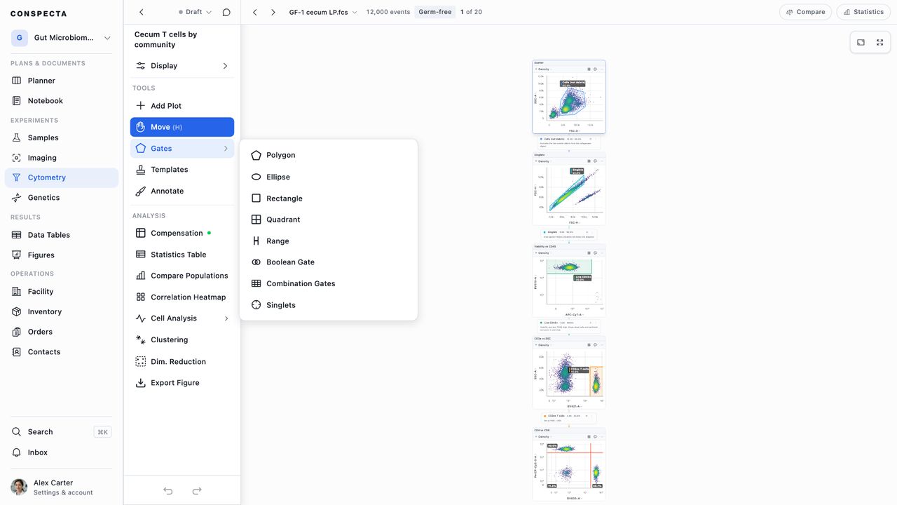
The Gates menu has three more tools.
Boolean Gate combines populations you already have with AND, OR, or NOT. Each population you select has a NOT toggle that flips it to its opposite, so "CD4-positive but not CD25-positive" is one gate.
Combination Gates counts every positive and negative pattern across 2 to 8 populations, such as CD4+ CD8-, CD4+ CD8+, and the rest, in one table. Use it for co-expression across a panel. It opens once the analysis has two populations to combine, and the row says so until then. A quadrant counts as its four corners.
- Pick the populations. Search by marker name or by the population a gate sits under. Pick the corners of a quadrant the same way as any other gate.
- Check Parent population. It starts on the population every gate you picked was drawn under, with its event count. It's the denominator for the percentages and the place the new gates go in the tree. Change it if you want a different one.
- Sort by Events to bring the rare patterns to the top. Empty patterns are hidden until you untick Hide empty.
- Tick the rows you want and click the create button, such as Create 3 gates, to make them all at once. To take the full table out without creating anything, click Copy or CSV.
If the gates you picked can't overlap, such as one drawn inside another or two corners of the same quadrant, the dialog box warns you. A zero in those rows comes from how the gates were drawn, not from the biology.
A combined population has no outline to draw, so each Boolean and combination gate gets a plot of its own, on the channels of the gates you combined. Tick more than 8 patterns at once and the gates land on their own, so the canvas stays readable. Read their counts in the Statistics Table.
Singlets finds FSC-A and FSC-H, draws the doublet-discrimination gate, and adds the plot if you don't have one.
What a Gate's Label Says
Each gate on a plot has a small label with its name and, under it, the percentage of its parent population inside the gate. While you drag the gate, the label shows an estimate marked with ~, and the exact number replaces it when you let go.
Two suffixes can follow the name:
- · this file means you changed the gate's boundary for the tube you're viewing, with Customize for this file. Its count differs from the same gate on your other tubes, and its outline is dashed. See Flow Files and Templates.
- · 2/3 means the gate could be placed on two of your three loaded files but not the third, usually because that file's panel is missing a channel the gate was drawn on. Check that file.
A gate placed on every file has no suffix.
When a plot has more gates than room for their labels, such as after you turn a clustering run into gates, some gates show only their name or a numbered marker. The number is the gate's place in the order the plot's gates were made. Hover over a marker or its gate, select the gate, or Tab to the marker to see its full label. When you export a plot that has markers, a key in one corner of the figure lists each number with its gate's name and percentage.
With the Move tool, you can drag a label anywhere on the plot and it stays there. It moves with its gate. To nudge a label, press Tab until it's selected, then use the arrow keys to move it a pixel at a time, or hold Shift to move it ten. To put a label back in its automatic place, open the gate's ⋯ menu and choose Reset Label Position. Moving a label leaves the gate's boundary and its numbers as they were.
Manage a Gate
On the arrow from a plot down to the plot beneath it, a small box shows the gate between them: its color, its name, how many events it kept (such as 10.5K events · 83.4%), and its note if it has one.
On a zoomed-out tree, click or tap the box to zoom in on it, with the plot above and the plot below in view. Its buttons work from there. From the keyboard, Shift + ↓ zooms in on the arrow below the selected plot and Shift + ↑ on the arrow above it.
- Click the box to see the gate's statistics.
- Click + to create a child plot from the population.
- Open the ⋮ menu for everything else.
The ⋮ menu lets you:
- change the gate's color
- Rename the gate
- add a note on why the gate sits where it does, with Add Note. Once the gate has one, Edit Note changes it in place in the box.
- Show Stats
- Lock Gate, so a stray drag can't move it
- New Plot, the same as +
- Export FCS to download the population as its own file
- Save population to project to keep it as a file in the project
- Delete Gate
- Customize for this file, when more than one file is loaded. It moves the gate on the tube you're viewing and leaves it in place on the others. Once used, it reads Reset to shared. See Flow Files and Templates.
Each of a quadrant's four corners gets its own box on the arrow, with the same menu, minus renaming, notes, and Delete Gate, which stay with the quadrant gate itself. Changing a corner's color recolors all four corners.
To name a corner, such as Tregs or Double negatives, choose Move and click the corner's percentage on the plot. Type the name and press Enter, or press Esc to leave it as it was. The name shows beside the percentage, on the corner's box and plot, and in the statistics and exports, where the corner's two conditions stay beside it: Tregs (CD4+ CD25+). Clear the name to go back to the automatic one. A template carries the names with it.
Deleting a gate also deletes every gate under it. The confirmation lists them first.
Save a Population as a New File
Save population to project saves the population as a new FCS file in your project, with a Name filled in from the gate and the source file. You can then work on that subset as its own dataset. The dialog box also offers to open a new analysis on the saved file, linked to the same sample as the analysis you saved from, and the analysis takes the same name.
The saved file records which analysis and gate it came from. Its row in the dataset's file table and its File Information panel both show Derived from, with a link to the source analysis. Derived from follows the source analysis's sharing, so only people who can open that analysis see it. The file itself is available to the whole project. Only the Derived from line is hidden, so a private analysis's gate names stay private.
Members with view-only access keep Export FCS but can't use Save population to project.
The Hierarchy
The tree of plots is your gating hierarchy. The plot beneath a gate shows that gate's population. The path above the plots shows the full route, such as All Events › Lymphocytes › CD3+ › CD4+. Click any step in the path to jump back to it.
To open a child plot under a gate, double-click the gate, or click + next to its name on the arrow below the plot.
A gate keeps counting the way you drew it if you remove its plot, add a second one beside it, or switch an axis to Log.
An older gate can show a banner that names it and says it's counted in an unconfirmed axis space. Treat its numbers as provisional until you add a plot back on the gate's two parameters, under the same parent gate.
Remove plot removes the plot and keeps every gate on it. If the plot is the last one showing a gate, Conspecta names that gate first. The gate keeps its numbers and stays in your statistics, with no plot showing it. The same warning names any older gate that reads its scaling from the plot you're removing. Removing a duplicated plot names its gates too, since those belong to that copy only.
Back-Gating
Open a plot's Plot style panel and find Backgate. It lists the populations gated beneath that plot. Turn any of them on to overlay it on the plot in a color you choose, and see where those cells sat on the original scatter.
Parameters
Click an axis label to change what it shows. The menu lists every channel in the file, then a Computed section for anything produced by clustering or dimensionality reduction, then the scale: Lin, Log, Logicle, or Asinh. Flow Visualization and Compensation covers what each scale does to a plot, and how to add more plots.
To give channels readable names, open Rename Parameters under Analysis → Cell Analysis. Rename FL2-A to CD8 PE once, and it reads that way on every axis, in every statistic, and in every export.
Keyboard
| Key | Action |
|---|---|
H R P E Q G | Move, rectangle, polygon, ellipse, quadrant, range |
A | Add plot |
F / O | Focus one plot, or fit the whole tree |
C | Compare the selected plot across every file |
1 to 9 | Select a plot |
| Arrow keys | Walk the hierarchy |
Shift + ← / → | Switch the active file |
Delete or Backspace | Delete the selected gate, unless it's locked |
Esc | Cancel or deselect |