Flow Cytometry Compute

Flow cytometry runs on your own machine by default, and that path consumes no compute usage. Gating, compensation, statistics, plotting, the specialized cell-cycle and proliferation tools, and every export are computed in your browser.

That's worth saying plainly, because most cloud analysis tools meter this work. In Conspecta you can re-gate a panel fifty times, run t-SNE, throw it away, and run it again, without anything counting against your team's allowance.

Clustering and dimensionality reduction are the two heaviest steps, and the only two the workspace lets you run on Conspecta's servers instead. A server run consumes usage. Leaving the setting on Local keeps it free.

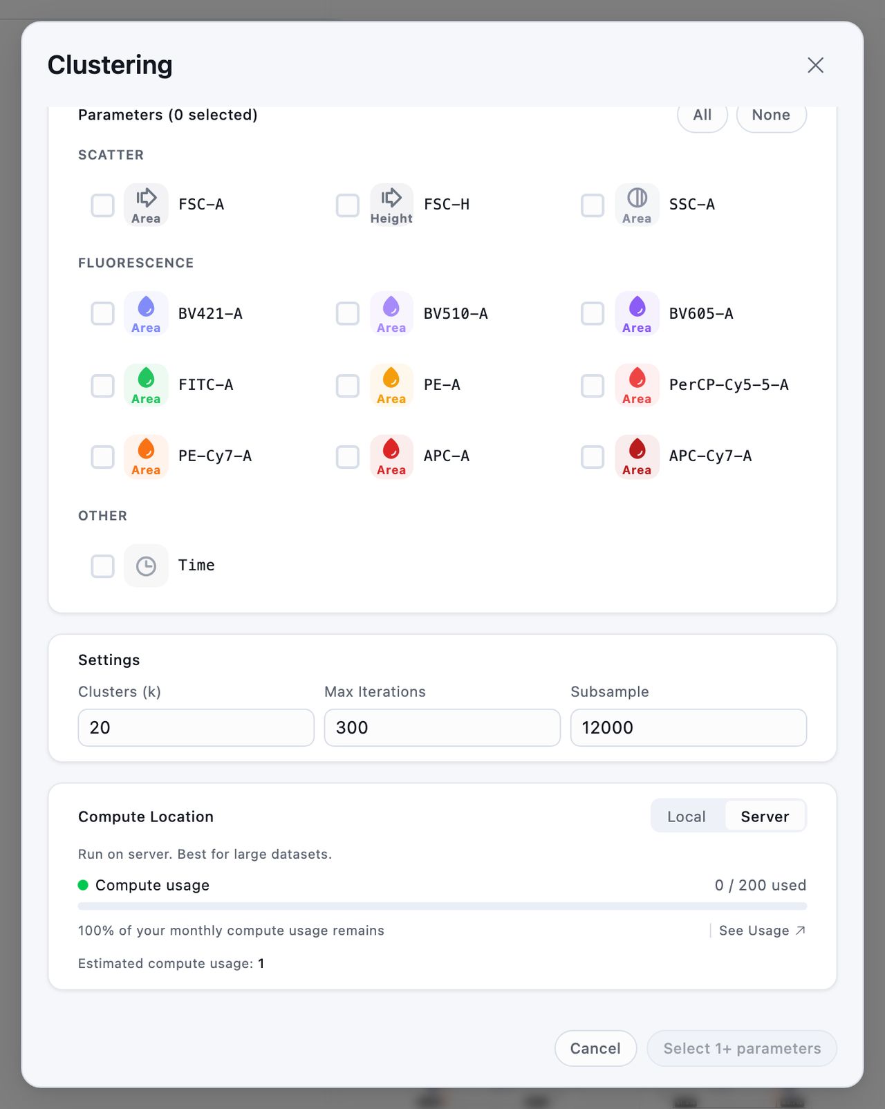
Choosing Where a Run Happens

Compute Location, in the Clustering and Dim. Reduction dialog boxes, has two settings. Local is the browser run, unchanged. Server hands the work to Conspecta's machines, which is the answer when the data is bigger than your laptop wants to chew through. A server reads the files out of your project's own storage, and a run can cover this file alone or the whole working set. A working-set run draws the same events, from the same files, in the same order a local run would, so the two give the same answer.

Every run starts on Local, however many events it covers, so nothing reaches a server unless you send it there. Pick Server before you press Run and the run follows what you picked.

Some runs are always local, and the dialog box says which case you're in instead of offering the choice:

• Density clustering. It reads one file's own density landscape, and only your browser runs it.
• A file that is still uploading. A server reads files out of your project, so there is nothing there to read until the upload finishes. For a working-set run, every file in the set has to finish.

What Uses Compute

The last two are there so an AI assistant connected to your project can work on your gates without you opening the workspace first. Both run the same code your browser runs and return the same numbers. Counting populations covers up to 512 MB of FCS data in one run, across at most 24 files. The limit is how much data the files hold, not how many there are, so two dozen small tubes fit in one run, and a run holding more is refused before any usage is charged, with a note of its total. Applying a gating strategy is free and covers up to 96 files in one apply (a full plate), because working out where each gate lands reads only the short header at the front of each file, never the events. An AI assistant can also start the server runs in the rows above, on one file of a saved analysis or pooled across several of its files at once, and those use exactly what the same run would use if you started it yourself. Reading a finished run back is free, and once a clustering run finishes, your AI assistant can save it onto the analysis. Opening the workspace later shows which algorithm ran, on which channels, what it found, and offers to re-run it to colour a plot.

What a server run uses comes from the algorithm alone: 1 for most of them, 5 for the two whose math takes minutes rather than seconds (DBSCAN and Graph clustering). That holds for a working-set run too, where covering ten files in one run uses the same as covering one. The size of your data changes how long a run takes, never what it uses. Every algorithm works on a sample of the events, so a five-million-event file and a fifty-thousand-event one cost the same. A server still never reads more than 500,000 events in one run: a single large file is strided down to that, and a working-set run whose per-file draw adds up past it is refused before any usage is charged, with the per-file number that would fit. The dialog box shows what the run in front of you will use, above what your team has left.

The Subsample setting changes how long a run takes, not what it uses. Usage is worked out from the file itself, so lowering the subsample on a server run finishes sooner and uses the same.

A server run can take up to 30 minutes. A run that would need more than that is refused when you start it, before any usage is charged, with a note about which settings to reduce. If the platform ever stops a run early, whether it hit the time limit or the server it ran on was interrupted, the run is marked failed and its usage comes back automatically.

Across the rest of Conspecta, usage is consumed by image analysis: running AI detection. Exports of every kind, including the flow export of your raw FCS files and gating, are free.

What This Means in Practice

A local run's ceiling is your laptop rather than a quota.

File loading is staged. A large file renders a 20,000-event preview immediately so you can start drawing gates, then swaps in the full resolution behind you. Statistics are always computed on every event, never on the preview.

Plots draw from a subsample. Scatter, density, and contour plots render up to 50,000 events, chosen once so the picture stays stable while you draw. Again, the numbers use everything.

How much you can hold is your machine's call, not a quota. A staged file costs no memory, so an analysis can cover a study far bigger than your RAM. Conspecta brings up to 200 files into the workspace at a time and moves the ones you haven't touched in a while out to browser storage, reading them back when you switch to them. Reopening a big analysis restores what fits in 200 files or 5 GB and tells you how many it left staged, ready to load from Manage files.

The heavy steps subsample by default. Dimensionality reduction and clustering both offer a subsample setting, pre-filled based on how many events you have, and tell you what fraction they're using. Lowering it is the first thing to try if a local run is taking too long.

Checking Your Usage

Settings → Usage shows your team's compute usage and a list of recent jobs. A server clustering run appears there with what it used. Flow exports appear with a usage of zero, so you can watch one finish without it drawing on your allowance.