Plasmid Maps and the Sequence Viewer
Open a sequence to see its map: the bases in rows, the features drawn over them, and the cut sites marked where the enzymes land. This page covers reading that map, the layers you put on it, the tools that run on a stretch of bases you pick out, and getting the picture into a paper.
The Three Views
Three buttons on the bar above the map switch between ways of drawing the same sequence.
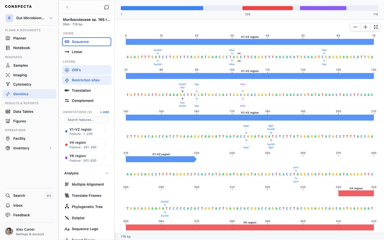
- Sequence shows the bases in rows with a ruler that counts from base 1 and annotation tracks, and it is where a linear sequence opens
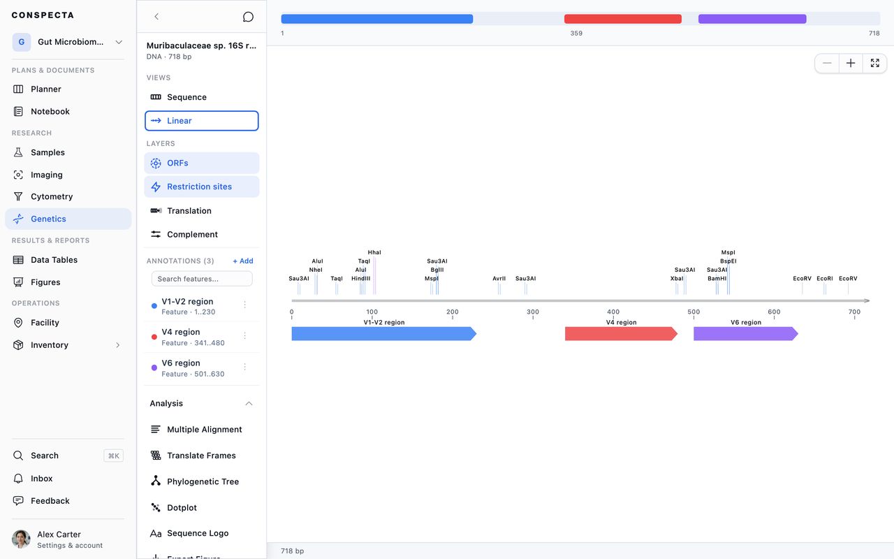
- Linear draws the whole sequence as a feature map
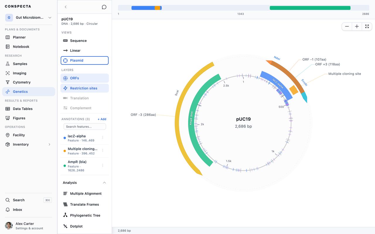
- Plasmid draws the circular map, and it appears for circular DNA and RNA sequences
A circular sequence opens on Plasmid, with its features drawn as arcs around the ring and its cut sites marked outside it.
Layers
Beside the view buttons sit the layers, which draw computed information over whichever view you are in:
| Layer | Default | What it draws |
|---|---|---|
| ORFs | On | Open reading frames on both strands, 100 amino acids and longer, each starting at a start codon and labeled with its frame and length, such as ORF +1 (243aa) |
| Restriction sites | On | The common enzymes, both strands, aware of circularity. Linear and Plasmid name the enzymes that cut once and mark every other site with a short, faint tick. The label reads (Scanning…) while it works |
| Translation | Off | Amino acids under CDS and gene features, including the ones the ORF layer found |
| Complement | Off | The reverse strand, under the bases |
Which layers you get follows the sequence type. ORFs and Translation apply to DNA and RNA, Restriction sites and Complement to DNA. A protein sequence gets no layer buttons at all, because every one of them reads nucleotides.
Translation and Complement gray out on Plasmid, where there are no base rows to draw them under. Switch to Sequence and they come back.
Moving Around
Cmd/Ctrl + F searches within the sequence, as text or as a regular expression, and steps through the matches with Prev and Next. Cmd/Ctrl + G jumps to a position on Sequence and Plasmid. Cmd/Ctrl + Z undoes and Cmd/Ctrl + Shift + Z redoes. Escape backs out of whatever is open, one layer at a time, and ends by clearing your selection.
Drag across the bases on Sequence to select a region. On Linear a drag moves the map, so hold Shift as you drag. On a phone or tablet, press and hold on the bases until the highlight appears, then drag, on either view. The status bar shows the selection's coordinates, length, GC content, reading frame, and, when the selection divides by three, how many amino acids it encodes. Plasmid shows the position under your cursor instead.
Working in a Selection
Dragging out a region opens a menu of tools that run on the bases you selected.
Picking an action closes the menu and keeps the region selected, so Selection tools in the status bar opens the same menu again for the next thing you want to run on those bases. Clear releases the selection.
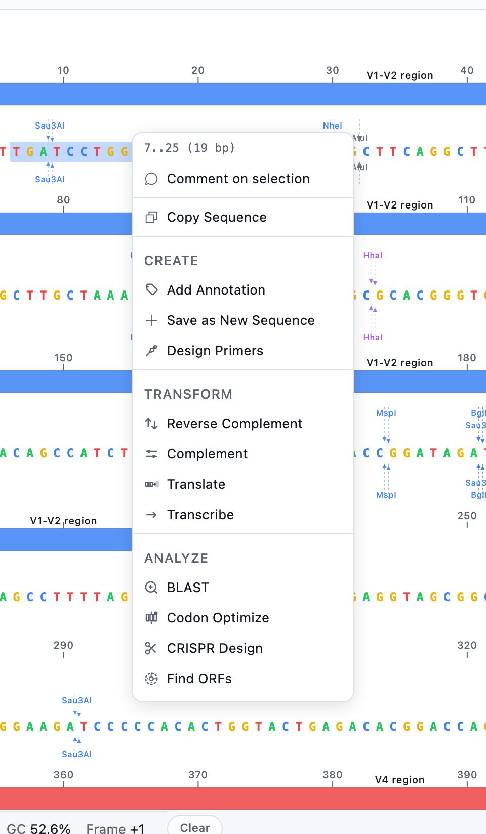
The menu opens with Comment on selection, which anchors a discussion to those bases, and Copy Sequence. Below them the tools sit in three groups:
| Group | On DNA | On RNA | On protein |
|---|---|---|---|
| Create | Add Annotation, Save as New Sequence, Design Primers | Add Annotation, Save as New Sequence | Add Annotation, Save as New Sequence |
| Transform | Reverse Complement, Complement, Translate, Transcribe | Reverse Complement, Complement, Translate, Reverse Transcribe | |
| Analyze | BLAST, Codon Optimize, CRISPR Design, Find ORFs | BLAST, Find ORFs | BLAST |
Save as New Sequence asks you to name the region before it writes anything, then confirms that it saved. From there you can Open sequence, or Keep working here to stay on the one you were reading.
The Transform tools and Find ORFs are covered in Sequence Analysis and BLAST, which also has BLAST. Design Primers, CRISPR Design, and Codon Optimize are in Primer and CRISPR Design. All of them open on the bases you selected.
BLAST, Design Primers, Codon Optimize, and CRISPR Design are also in the Analysis menu at the top of the sidebar, under Compare and Design. Opened from there with nothing selected, each one runs on the whole sequence.
Features
Add beside Features in the sidebar, or Add Annotation in the selection menu, opens the annotation editor. It takes five things:
- A Label
- A Start and End
- A Direction of Forward, Reverse, or None
- An optional note
- A Type, one of nine: Gene, CDS, Promoter, Terminator, Origin, Primer Binding Site, Restriction Site, Feature, and Custom
Each type carries its own color onto the map, and Custom is one of those nine presets, picked from the list like the others.
Auto-Detect, in the header of that dialog box when you are creating an annotation on a DNA sequence, opens Auto-Annotate Features. It scans against a library of common parts (T7 and lac promoters, rrnB and T7 terminators, resistance markers, reporters, origins, epitope tags, and ribosome binding sites), then lists every hit for you to tick. Select all ticks every hit. The hits you ticked go on the map when you press Add.
Features in the sidebar, under the tool menus, lists every one with its type and coordinates under a search box. Once there is more than one kind, the filter button at the right end of the search box narrows the list to one type, and shows how many features each type has. Each row's menu holds Edit, Hide or Show, and Delete. A hidden feature stays in the list, dimmed.
Click a feature's row in Features, or its block on the bar above the map, to select it. The selected feature keeps its full color and gains an outline while every other feature fades, on the bar and in all three views. Click the row again, or an empty part of the map, and they all come back.
Narrow the window and the sidebar becomes a column of icons. The tool menus keep their place at the top, and the list opens from the feature icon under them.
Tip: Select an annotation and press Delete to
remove it. Every delete shows Undo for a few seconds, and
Cmd/Ctrl + Z undoes adding, editing, and deleting annotations.
Exporting a Figure
Export Figure, in the actions menu at the right of the bar above the map, writes the view on screen, whether that is the circular map, the linear map, or the sequence rows.
Four settings shape the file:
| Setting | What it offers |
|---|---|
| Format | SVG or PNG |
| Width | The printed width, as Fits one journal column (89 mm), Fits both journal columns (183 mm), Fills a presentation slide (254 mm), or a Custom width anywhere from 10 to 1000 mm. It starts on both journal columns |
| Resolution | 150, 300, and 600 DPI, starting at 300 |
| Theme | Draws the map Light or Dark, starting on Light whichever theme the app is in |
Choose SVG and the map is drawn as shapes, with feature arrows, the backbone, tick marks and every label as separate objects and the feature names as text you can retype. Open it in Illustrator or Inkscape to recolor one feature without touching the rest. It prints at the width you picked whatever the resolution, because a resolution setting applies only to pixel images.
Choose PNG and the map is captured at the resolution you picked, then opened with two tabs: Export downloads or copies it, and Annotate draws arrows and labels on it first.
The figure carries whatever the map is showing, so the layers you switched on come with it: ORFs, restriction cut sites with their enzyme names, the amino acids of a translated feature, and the complement strand.