Flow Files and Templates
A Cytometry analysis holds one gating strategy and applies it to every file in it. This page covers grouping files into conditions, comparing them, and saving a strategy as a template for the next experiment.
Apply One Gating Strategy to Many Files
An analysis has a single set of gates that applies to every file in it, drawn the way Analyze Flow Cytometry Data describes. Conspecta matches gates to each file by channel name, so a panel acquired with the detectors in a different order still lines up.
When staining varies enough between tubes that one boundary won't do, you can move a gate on a single file without moving it everywhere. With more than one file loaded, Customize for this file on the gate's ⋮ menu unlinks that gate on the file you're viewing, and dragging it from then on adjusts only that copy.
That gate then has a dashed outline and its label reads · this file, so you can see which counts came from a gate you moved. Reset to shared puts it back on the shared boundary and discards the tailored one.
Files exist in three states:
- Attached to the analysis, so they're part of it
- Loaded, meaning in memory and ready to plot
- Not loaded, meaning attached but not in memory
The bar above the plots shows which sample you're looking at and where it sits in the analysis, such as 14 of 96, with the number of files not loaded beside it. Use the arrows, or Shift + ← and Shift + →, to move to the previous or next sample.
Click the sample's name to see every file, grouped by condition. You can search the list by filename, sample name, or tube name.
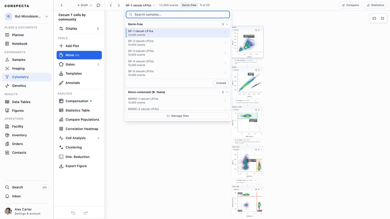
At the bottom of the list, Load all loads every file that isn't loaded and shows their total size. While they load, the button reads Loading 6 of 24.
Manage files, at the bottom of the same list, is where you attach files from your datasets, upload new ones, and choose which are loaded. Once an analysis holds more than a handful, Filter files at the top narrows the list by filename, tube name, or the sample a file was acquired from.
From datasets, on the right of Manage files, lists the project's datasets. To add a whole dataset, such as a run's single-stain controls, press Add all 10 on its row and pick a condition, Unassigned, or New condition from this dataset, which makes a condition with the dataset's name and puts its files in it. Files already in the analysis are left out of the count, and the button goes once every file is in.
To add only some of a dataset's files, click the dataset to open its file list. Tick the files you want, or use the checkbox beside the dataset's name to select every file not yet in the analysis, then choose where they go from Add 9 to in the bar at the bottom. Files already in the analysis are marked Attached, and All datasets takes you back to the list.
Tip: An analysis can hold more data than your computer's memory. A file that isn't loaded costs no memory, so load the files you're working on and unload the rest. When you reopen a large analysis, it loads up to 200 files or 5 GB and tells you how many it left unloaded.
Conditions
A condition labels what a file is: treated or untreated, day 0 or day 7, patient or control. Conditions group the rows of the aggregate statistics table, set the default grouping in the compare view, and let Conspecta test for significant differences between groups.
A file belongs to at most one condition, and files with none sit under Unassigned.
Creating Conditions
Click + New condition on the Conditions bar in Manage files, type a name, and press Enter.
When your file names already carry the groups, such as GF-1, GF-2 and SPF-1, Manage files suggests conditions above Unassigned:
- Click Review 4 conditions (the number is how many it found) to see each group with its files.
- If it split the names in the wrong place, pick another part of the name under Split by.
- Name each group, and untick any you don't want.
- Click Create 4 conditions. Each group's files move into its new condition. Files in an unticked group, and files that fit no group, stay where they are.
Moving Files Between Conditions
In Manage files, there are four ways to put a file under a condition:
- Drag its row onto the condition you want.
- Open the row's ⋯ menu and pick Move to the condition by name.
- Select several files and click Move in the bar that replaces the Conditions bar while they're selected.
- Use the arrows on a row to send it to the band above or below.
In the sample list above the plots, each row's ⋯ menu has Move to as well, and you can drag rows between conditions there too.
Loading a Condition's Files
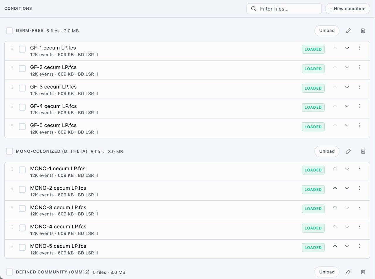
Files that aren't loaded stay under their condition, dimmed, in both the sample list and Manage files. To compare two conditions from a large study, load those two and unload the rest. Fewer loaded files also keeps gating quick.
| To | Do this |
|---|---|
| Load or unload a whole condition | Press Load or Unload along the bottom of its card in the sample list, or in its header in Manage files. Load shows the size, such as Load 3.1 GB |
| Load one file | Click it in the sample list, or press Load on its row in Manage files |
| Unload one file | Pick Unload from its row's ⋯ menu |
| Load or unload several | Select them in Manage files and press Load or Unload in the bar above the list. The checkbox beside a condition's name selects every file in it |
If the file an analysis opens on can't be loaded, the plot area says why, and your gates and plots stay saved with the analysis. Choose another file opens Manage files when the file was permanently deleted or can't be read as FCS. Try again fetches it again when the download stopped partway.
Comparing Across Files
There are three ways to look at more than one file.
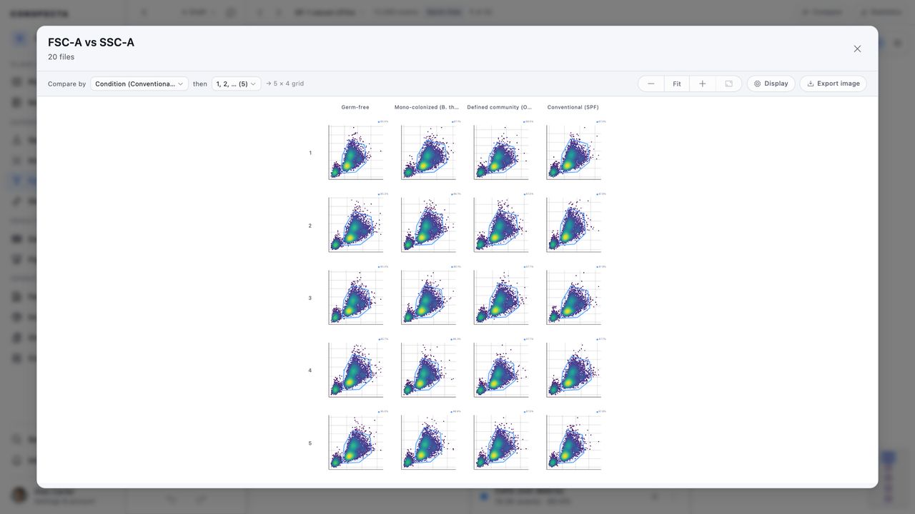
Compare all files (C, or the grid button on a plot) takes one plot and draws it for every loaded file at once, which is how you check that the gate sits right on every file. On a plot with nothing to its right in the gating tree, → opens it too, and ← closes it again.
Group the grid by condition, tube name, experiment, cytometer, acquisition date, plate, well row, well column, or a segment of the filename, then group again within that. Files acquired on a plate loader carry their well, so grouping by well row and then well column lays the panels out the way the plate sat, with rows down, columns across, and an empty square wherever a well was skipped.
Display sets whether each panel shows gates, population statistics, axis labels, and file names. When the grouping already tells you which file each panel is, file names are hidden to give the plots more room. Turn File names back on under Display to show them anyway, and they stay on while you regroup.
A grid has room for one file per square, so replicate files, and files missing either value, are left out. A note next to the grouping controls says how many were left out and why. Open it to see which files, or switch to grouping by one field to show them all.
Make the panels bigger to read one closely, or choose Fit to see them all again.
Export image opens the grid with two tabs: Export sets the format, size, and file name and downloads or copies it, and Annotate marks it up first.
Compare on the sample bar applies your gates to the files you pick and shows a Batch Statistics table of counts and percentages. The files are listed by condition, as in the sample list. The checkbox beside a condition's name picks every loaded file in it, and Load at the bottom of its card brings in the rest. It needs at least one gate and two loaded files, and it lists any file where a gate couldn't be placed.
Statistics, next to it, opens Aggregate Statistics. Rows are files, columns are populations, and cells are percentages of parent. A quadrant gets a column for itself and one for each of its four corners, so you can compare a double-positive frequency across files. With conditions assigned, the table adds:
- Each condition's band ends with a mean ± standard deviation row
- A cell more than two standard deviations from its band's mean is flagged
- With exactly two named conditions and at least two files in each, a Welch's t-test row appears, with p-values corrected for multiple comparisons and significance marked
- Below the table, a row of per-gate dot plots shows every file as a point, ordered so the most significant gate comes first
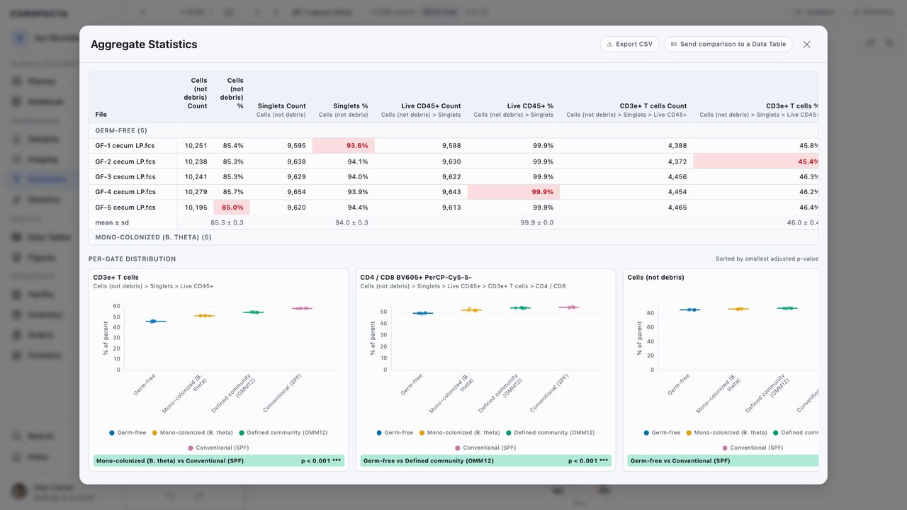
From there you can Export CSV or Send comparison to a Data Table.
Dose-Response Curves
Name each condition for the dose it received, with its unit, and a Dose-response section appears under the dot plots with one card per population. Each card plots every file against dose on a log axis, draws the fitted four-parameter logistic curve through them, and reports EC50 with the Hill slope, the top and bottom plateaus, and R². A response that falls with dose reads as IC50 instead. The grid button on a card puts that chart on a figure, curve included.
A condition counts as a dose only when it carries a unit, so "10 nM" fits a curve and "10" on its own does not. A curve needs at least four dose levels, and every condition has to carry the same unit. The zero-dose arm is plotted a decade below the lowest nonzero dose, because a log axis has no position for zero. Files left in Unassigned sit out of the fit.
The population with the best fit comes first. A poor fit shows the R² instead of an EC50, and an EC50 that falls outside the doses you ran is marked as a projection. If a condition's name can't be read as a dose, the section names it so you know which one to rename.
Gating Templates
A template is a gating strategy you save so you can use it again on other files. It holds the gates, the plots they're drawn on, and the compensation matrix they were drawn with.
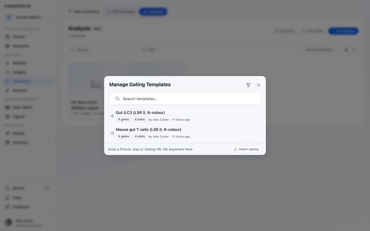
Open Your Templates
Every template in the project is in one list, and you can open it from two places:
- In an analysis, click Templates in the sidebar. This is where you save, apply, and import templates.
- On the Flow Cytometry page, open the Analysis tab and click Templates at the top. Use this to manage templates, or to import one before you have any data.
Search the list by name, or pick one from Recent at the top.
Save Your Gating as a Template
Once you've drawn at least one gate, open Templates in the sidebar and click Save current gating as a template at the top of the list. Give it a name and, if you like, a description. Conspecta shows what the template will include before you save it.
Import Gating from FlowJo
Conspecta reads the gating in a FlowJo 10 workspace (.wsp) or a Gating-ML 2.0 file (.xml or .gml), the format Cytobank and the R CytoML package write. Drag the file onto any of these:
- An open analysis, once a file is loaded in it
- The FCS Datasets or Analysis tab of the Flow Cytometry page
- The list in Templates, which also has an Import gating button if you'd rather pick the file
Conspecta reads the file in your browser and shows you the gates it found before saving anything. Any gate it couldn't rebuild is listed with the reason. The cell counts on this screen are the ones recorded in the original file.
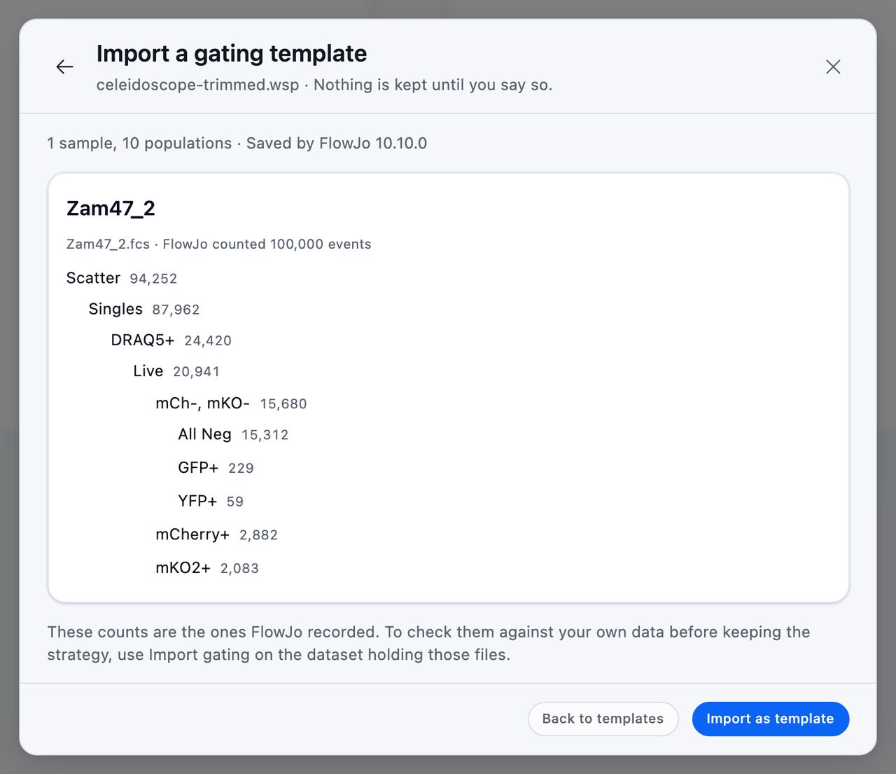
Click Import as template to save it, or Import 3 templates for a file with three samples. Each sample in the file becomes its own template. When the file has one sample, its template opens next, and in an analysis you can click Apply template to use it. When it has several, you go back to the list to choose one.
A workspace from FlowJo 9 or earlier won't open. Save it again in FlowJo 10 and import that copy. A Gating-ML 1.5 file needs exporting again as Gating-ML 2.0.
To check the gating against your own FCS files before you keep it, open the dataset that holds those files and use Import gating in its ⋮ menu. That import runs the gates on your data and compares the counts with the ones in the file, population by population. Checking a workspace against your data covers it.
Find a Template That Fits Your Files
In an analysis, a template that uses a channel your files don't have shows a warning on its row, such as Missing CD4. No gates fit means none of its gates can be placed on your files. A row with no warning will apply cleanly.
To narrow the list, click the filter icon next to the search box. You can show only templates that fit your files, approved templates, or templates you created, and combine them.
What's in a Template
Click a template to open it. It has three tabs:
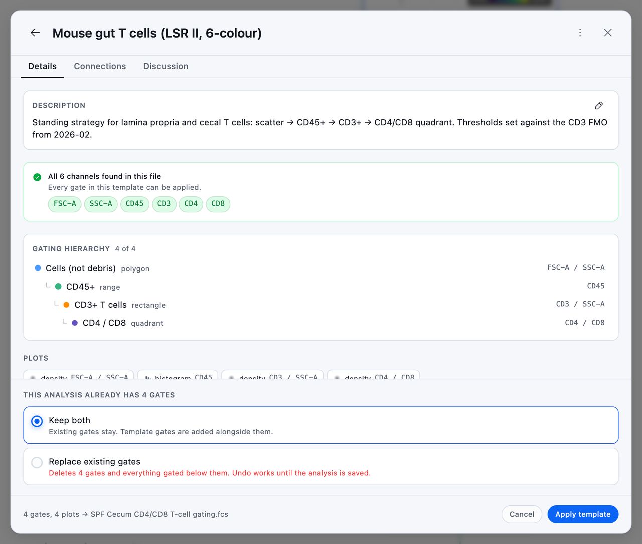
- Details shows the gates, the plots, and whether the template fits the files you have open. You can add or change the description at the top whenever you like.
- Connections shows every analysis built from the template, with the template version each one used. An analysis on an older version is marked behind latest. Click an analysis to open it, or click any item on the map to see what that item connects to, such as the files an analysis used.
- Activity has comments and sign-offs alongside the template's history of changes. Use it to agree on a standard panel with your lab.
Export Templates
To send a template to someone who uses FlowJo or another tool, open it and use the ⋮ menu:
- Export as FlowJo .wsp saves a FlowJo 10 workspace.
- Export as Gating-ML saves an
.xmlfile that FlowJo, Cytobank, and the RCytoMLpackage can open.
If a gate can't be written in the format you chose, it's left out and listed with the reason.
To export several templates at once, click Export on the Analysis tab and choose The gating templates. It starts with the templates behind each analysis you're exporting. Set Scope to Every template to include the rest. The same dialog box can export The gating strategy of each analysis too.
To export every template in the project, go to Settings → Export, tick Gating Templates, and choose Gating-ML. You get a zip with one file per template and a spreadsheet of versions and sign-offs. Tick Flow Analysis to do the same for every analysis.
Apply a Template
When you open a template in an analysis, Conspecta checks it against every file in the analysis before you apply it. You see which gates will be placed, which can't be because a channel is missing, and which are skipped because the gate above them can't be placed. Missing channels are listed for each file. Gates that can't be placed are left out when you apply.
Then choose how to apply it:
- Keep both adds the template's gates next to the ones you already have. This is the default.
- Replace existing gates deletes your current gates, and everything gated under them, before adding the template's.
Replace existing gates deletes your current gating. A template that includes a compensation matrix also replaces the analysis's compensation, whichever option you choose. Undo works only until the analysis saves, so if you're unsure, choose Keep both and delete what you don't need.
Templates belong to the project, so everyone on it sees the same list. Members with view-only access can open templates, read the discussion, and export them. Saving, applying, importing, and editing templates need edit access.
If a teammate changed the same thing while you used Rename, Edit description, or Update with current gating on a template's ⋮ menu, the box you were working in shows both versions under Keep mine and Use theirs, and Apply keeps the one you pick. A teammate's change to another part of the template goes through alongside yours.
Re-Apply a Newer Template Version
Conspecta records which version of a template an analysis used. If someone updates the template later, the analysis details show that the analysis uses an older version and offer to re-apply the latest. Your gates don't change until you re-apply.
Quality Control
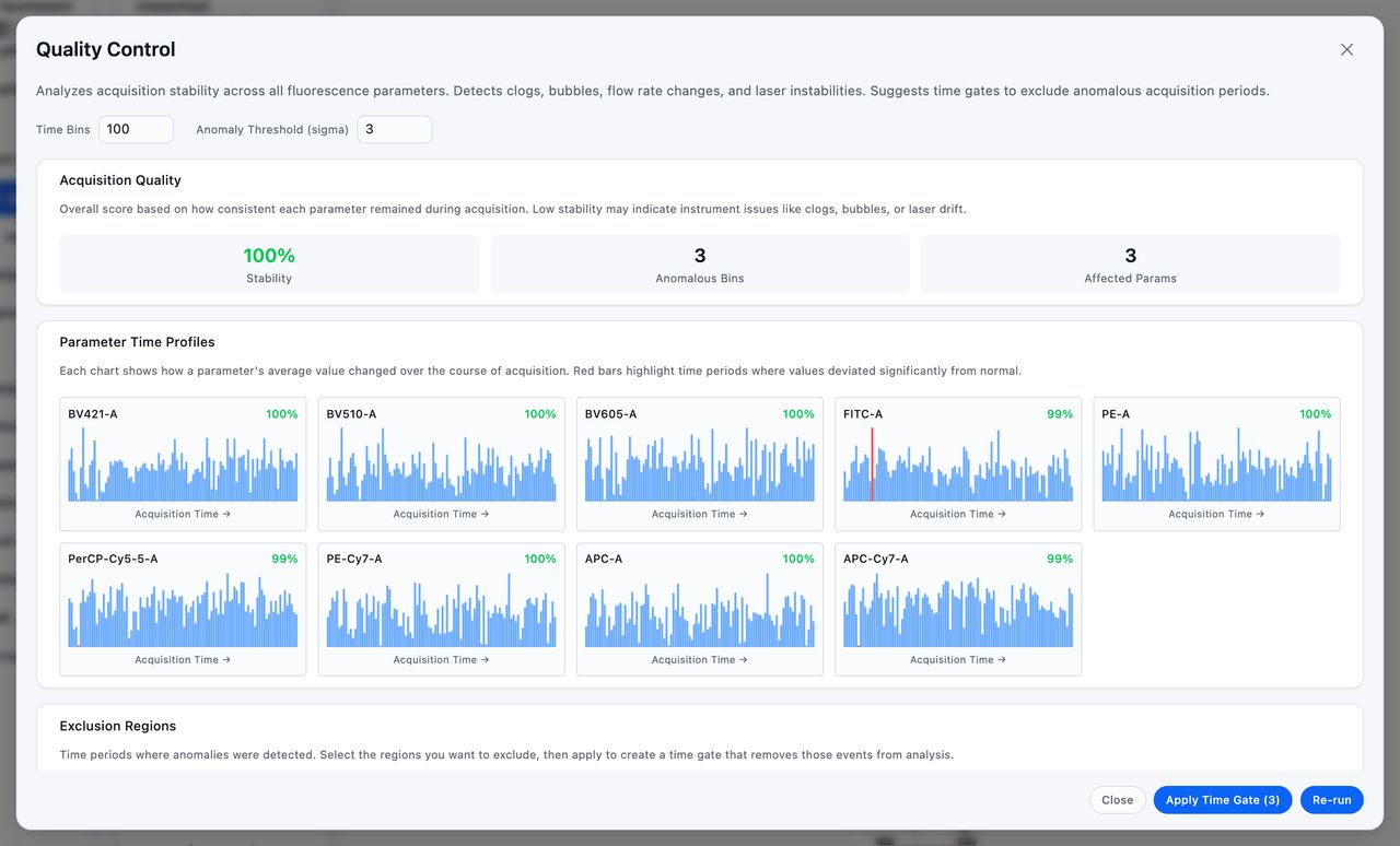
Quality Control, under Analysis → Cell Analysis, looks for instability during acquisition, such as a clog, a bubble, or a pressure drift. It bins the run by time and flags bins that sit outside your threshold, defaulting to 100 bins and 3 standard deviations.
Review the flagged regions, deselect any you're happy with, and press Apply Time Gate. A green dot marks the filter as active.
Applying a time gate re-parents your whole tree. Conspecta creates a gate named "QC Time" covering the good time windows, draws it on a Time histogram at the top of the tree, and moves every top-level gate and plot underneath it, so all your existing populations are now filtered by it. Applying again replaces the earlier "QC Time" gate. One undo takes the whole apply back. Removing the filter later clears the result without deleting the gates it made.
Quality control needs the file to carry a TIME channel.