Sequence Analysis and BLAST
These tools read a sequence and report what it matches in the public databases, what it looks like on the other strand or in another frame, how it lines up against your other sequences, and what a protein or an RNA is likely doing structurally.
You reach these tools in two ways. Analysis, at the top of the sidebar, opens a menu of everything that applies to this sequence, so a protein offers the protein tools and an RNA offers RNA structure. Dragging out a region on the map opens a menu of its own, covered in Plasmid Maps and the Sequence Viewer. BLAST, Design Primers, Codon Optimize, and CRISPR Design are in both, and run on the whole sequence when nothing is selected.
The Analysis menu groups its tools by the question they answer:
| Heading | What it holds |
|---|---|
| Compare | BLAST, Multiple Alignment, Dotplot, Sequence Logo, Phylogenetic Tree |
| Design | Design Primers, Codon Optimize, CRISPR Design, on DNA |
| Read | Translate Frames on DNA and RNA, RNA Structure on RNA, and the three protein tools |
BLAST
BLAST searches your selection against NCBI, or the whole sequence when nothing is selected. It is under Compare in the Analysis menu, and in the selection menu.
Three settings shape the search:
| Setting | What it takes |
|---|---|
| Database | Nucleotide (nt), Protein (nr), or SwissProt, starting on the one that matches your sequence |
| Program, below it | Worked out from that choice and your sequence together |
| Max Results | 10 to 100 hits, starting at 50 |
The Program follows the database:
- nt runs BLASTN whatever you give it.
- nr or SwissProt run BLASTX on nucleotides and BLASTP on protein.
Hits come back as a sortable table of accession, name, organism, identity, E-value, bit score, and alignment length, sorted by identity. Open a row for the full name, the record's own length, and the raw score.
Saving a hit fetches the full annotated record from its accession and adds it to your library at once, named for its accession and organism, with the sequence you searched from recorded as its parent.
Sequence lookups leave Conspecta for NCBI and UniProt. Every screen that sends one carries a notice saying so. A BLAST search sends your whole query sequence. Fetching a record by accession, searching by keyword, and saving a BLAST hit send the accession or the words you typed. All of them go through our servers, so the address those databases see is our server's. Nothing else from your project goes with any of it, and no account, project, or contact details are sent. Avoid searching sequences you need to keep unpublished.
Transforming a Selection
The Transform group in the selection menu shows the bases you picked rewritten, and leaves your sequence as it is. Reverse Complement, Complement, and Translate are there for DNA and RNA, Transcribe for DNA, and Reverse Transcribe for RNA.
Find ORFs, under Analyze, scans all six frames of your selection for open reading frames of 30 amino acids and up, whether or not they start at a start codon, and lists them longest first with their frame, strand, position, and whether each has a start and a stop. That is a looser search than the ORFs layer on the map, which only draws frames of 100 amino acids and up that begin at a start codon, so the tool will find things the map does not draw.
Every result numbers its positions against the whole sequence, not against your selection.
A single-sequence result, such as a reverse complement or a translation, has Copy and Save as new sequence underneath it. Saving asks for a name and offers Open sequence. The original is untouched, and the new sequence records where it came from.
Find ORFs and Translate Frames produce a list, so each row carries its own copy button.
Aligning Sequences
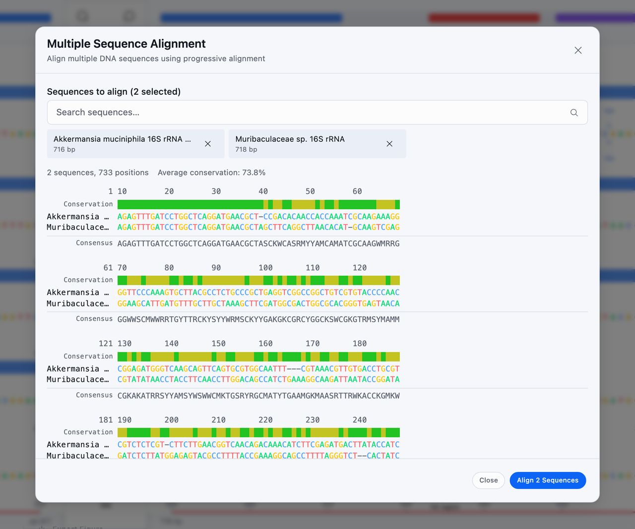
Multiple Alignment, under Compare, lines this sequence up against others you pick. Only sequences of the same type are offered, and you need at least two. Pick a folder to add every sequence of that type inside it, including those in folders within it. Conspecta builds a guide tree and merges the sequences along it, pairwise, which is the standard progressive approach.
The viewer breaks the alignment into blocks of sixty columns, each with its own position ruler, a conservation bar colored from red to green, one row per sequence, and a consensus row underneath. Above the blocks it reports how many sequences and positions there are, and the average conservation across them. Hover any column of the bar to read what fraction of the sequences agree there.
Translate Frames shows all three forward reading frames of the whole sequence at once, each with its length and where it stops.
Checking a Sequence Against Sanger Reads
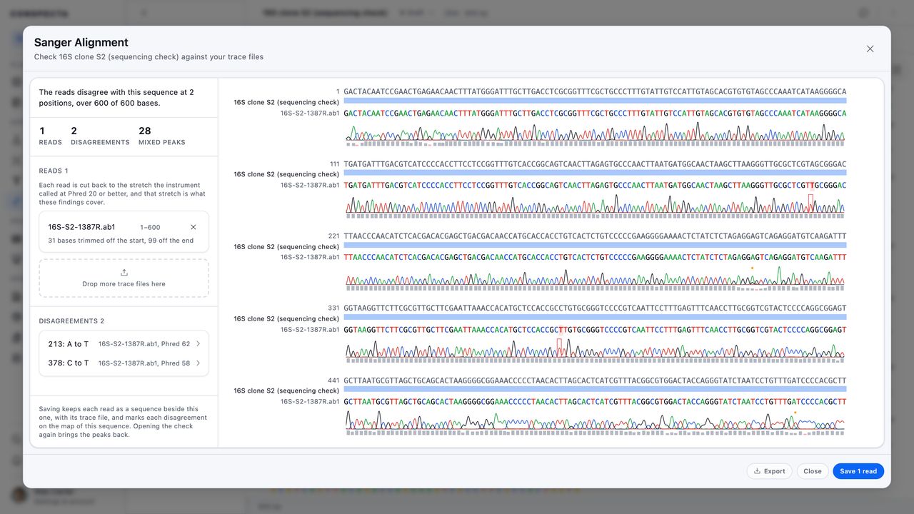
Sanger Alignment, under Compare, checks this sequence against the trace files your sequencing service sent back. Drop the .ab1 files onto the dialog box, or choose them, up to 96 at a time.
Trimming and Placing Reads
Each read is cut back before it is checked against the sequence. The first few dozen bases of a capillary run are noise, and the end of the run degrades the same way, so only the stretch the instrument called at Phred 20 or better is judged. The reads list says how many bases came off each end, and every count on the panel covers what was kept. A read that never rises above that line anywhere is listed as unplaced, with that as the reason.
Each read is placed where it belongs on the sequence and drawn with its chromatogram underneath, so a base that disagrees and the peak that produced it are in one view. A read from the reverse primer is flipped for you and reads left to right with the rest. Positions where a second base is up alongside the called one are marked, which is what a heterozygous site or a mixed population looks like in a trace.
The reads have to belong to this sequence. One that lines up with nothing is listed as unplaced, which usually means the wrong reference.
Reading the Findings
Beside the drawing is the same information as text, in a panel with a section for each part:
- What the reads found
- The reads that were placed and the stretch each one covers
- Every disagreement with its position and the read's own confidence there
- Any read that could not be placed, with the reason
Click a disagreement to jump the view to it.
Clicking a disagreement also rings that base in the sequence, in the read, and on its trace, and opens a panel with its peaks drawn large. The panel shows a dozen bases at a time, the sequence over each read's call with the peaks beneath them, and a slider that walks the whole construct. Previous and Next jump between the disagreements. On a wide screen the panel sits beside the drawing, and on a narrower one above it. Close it to give the drawing its room back.
On a phone it splits into two tabs. Findings is the panel above. Trace is the same view of the peaks, and tapping a disagreement under Findings opens it there.
Files that arrive later go in through the drop target under the read list, or by dropping them anywhere on the dialog box. Each read in that list carries a control to take it back out. It asks first, then checks the sequence against the reads that are left.
Exporting and Saving a Check
Export writes the view as SVG, PDF, PNG, or TIFF. The PDF and SVG are vector, so the peaks stay sharp at any size. Theme draws it Light or Dark.
Save puts each placed read into the workspace as its own sequence, in the same folder as the sequence it was checked against, and stores its trace file with it. Each one carries its per-base quality and points at that sequence, so Connections shows what was sequenced against what.
The sequence's card in the workspace then draws the read coverage and says what the reads confirmed, and its map marks each disagreement on the base itself, in Text, Linear, and Circular. Click a mark to open Sanger Alignment at that base, with the reads and their peaks already loaded.
Opening Sanger Alignment from Compare on a checked sequence loads them the same way, and dropping more files adds to the check. Saving again adds only the new reads.
A check saved before trace files were stored opens on the names of the files it was run with, and dropping them again brings the peaks back.
Trees, Dotplots, and Logos
Phylogenetic Tree builds a UPGMA tree from sequences you pick, or from every sequence in a folder you pick. It accepts a mix of sequence types, so check what you selected before reading anything into the topology. Download SVG writes a vector file, with branches as lines and tip labels as text you can edit in Illustrator, and Copy Newick copies the tree to the clipboard.
The Import Newick tab reads a tree someone sent you. Paste it in, or use Upload File to read a .nwk, .tree, .newick, or .txt into the box, then press Import Tree to draw it.
Dotplot compares this sequence against one other and draws where they match. Window Size runs from 5 to 25 bases and starts at 11, and Match Threshold runs from 50 to 100 percent and starts at 70. Underneath the plot you see the number of matches, how many diagonal runs there are, and the longest one, which together show whether the similarity is one colinear stretch or scattered noise.
Sequence Logo draws the conservation of several sequences as stacked letters, with the y-axis in bits. It needs at least two sequences of the same type and the same length, since it reads column by column and does not align for you. Run Multiple Alignment first and use the result.
RNA and Protein Structure
RNA Structure, on RNA sequences, folds the sequence to maximize base pairs and draws the result as an arc diagram, as dot-bracket notation, and as a list of stems and loops. Min hairpin loop sets how tight a turn is allowed, from 1 to 5 bases, and starts at 3. Allow G-U wobble pairs is on. The Pairing score it reports is a count of pairs, not a free energy, so use it to compare foldings of the same sequence.
Three tools read proteins:
| Tool | What it gives you |
|---|---|
| Hydropathy Plot | A Kyte-Doolittle trace over a window you set from 5 to 21 residues, the overall GRAVY value, and the stretches hydrophobic enough and long enough to be called as likely transmembrane regions |
| Protein Properties | Isoelectric point, net charge at pH 7.4, extinction coefficient at 280 nm both with cysteines reduced and with them paired, the matching A 0.1% values, the Trp, Tyr, and Cys counts behind them, and molecular weight |
| Secondary Structure | A Chou-Fasman prediction as helix, sheet, and coil percentages, a colored map along the sequence, propensity plots, and each predicted region with its span and score |
A protein with no tryptophan, tyrosine, or cysteine gets a note in place of an extinction coefficient, because nothing in it absorbs at 280 nm.